
Automatic compensation banks
During previous decades manufacturers of automatic compensation banks faced increasing competition worldwide. They were forced to produce as economically as possible. Now, new technologies have been developed compared with the past when capacitors were bigger and heavier.
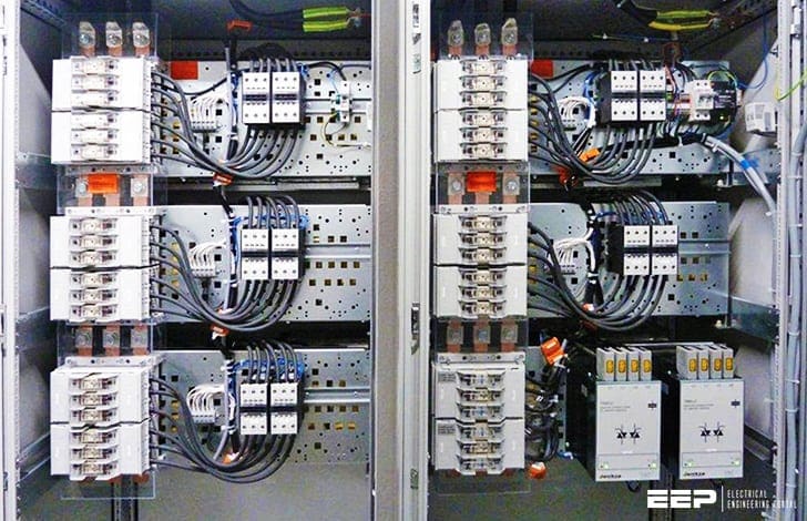 Installing and setting into operation of automatically controlled compensation bank
Minimizing capacitors enabled the development of steps (modules containing capacitors) with discharging resistances, fuses, contactors and reactors (if required) assembled in standardized industrial cubicles.
Power factor relays are usually fitted in the doors. Due to reduced active power losses inside the capacitors, today it is possible to assemble compensation banks up to 400 kvar or more within one cubicle of dimensions (B × H × W) = 600 mm × 2000 mm × 400 mm (without reactors).
Let’s discuss now installation and setting into operation of LV automatically controlled compensation banks:
1. Installation requirements
First of all, national directions regarding the installation of electrical power plants up to 1000V rated voltage must be checked. European standards, described in EN 60931-1 and 3 for instance, prescribe rules for the installation of capacitor banks valid for many countries around the world.
Before installing a new automatically controlled compensation bank the technical data have to be checked to see whether the bank complies with the requirements listed in the individual orders, such as:
- Is the rated voltage identical to or higher compared with the nominal voltage of the grid?
- Is the rated reactive power sufficient for the application, and even extendable if required?
- Does the admissible ambient temperature compare with the real one?
- If reactor protected, is the reactor rate identical to the ordered one?
- Does the integrated power factor controller fulfil the input data with reference to the external current transformer? Are free steps available for extension?
- Is the space for locating the bank sufficient, dry and not too close to heat-emitting devices?
- Is the location free of vibrations (if not, the bank is to be set on gum buffers)?
- Are the technical data of the compensation bank always visible?
Further, an additional plus tolerance of the capacitor’s capacitance must be considered in the range of up to 10%. These factors (1.3 × 1.1) result in an overcurrent of Io = 1.43 × In. Roughly determined, the cross-section of cables and conductors should be selected according to 1.5 times the nominal current.
This overload capability together with the high inrush current to the capacitors must be taken into account when designing protective devices and cable cross-sections.
Table 1 (click to open) lists nominal currents, cable cross-sections and fuses belonging to capacitors or banks of different nominal reactive power applicable for grids’ nominal voltage levels of 230, 400 and 525 V.
Thus a compensation bank with a rated reactive power of 100 kvar at a nominal voltage of 400 V, for instance, has a 144 A nominal current, which, when multiplied by 1.43, results in 200 A approximately. According to Table 1, a cross-section of 3 × 95/50 mm2 is then necessary.
2. Setting into operation of automatic compensation banks
Figure 1 shows the principal circuit diagram of an automatic compensation bank. The bank itself delivered by the manufacturer is entirely wired up and ready to connect.
The main work for the electricians is to connect the bank with the selected power cables to the distribution plant. The provided fuses or load circuit breaker must comply with the specifications described above.
Further, a cable with a cross-section of at least 2×2.5 mm2 is to be laid from the measuring current transformer to the power factor controller in the automatic compensation bank. The cross-section depends on the distance between them of course and is illustrated graphically in Figure 2a,b for current transformers both with nominal secondary outputs of either 5 A or 1 A.
Selection of CT and determination of the CT cable
Most existing electrical distribution plants already have CTs fitted. First of all, it is necessary to check the transforming ratio and then, second, the nominal burden. These two criteria are essential for proper control of reactive power.
An admissible minimum of power factor controller sensitivity should not undersize 1% of the nominal secondary current of the CT. This results in 0.05 A or 0.01 A reactive referring to the nominal secondary current of the CT, either 5 A or 1 A, respectively.
Incidentally, if the step size is, for example, 10 kvar, proper control by the power factor controller is no longer possible. In this case a separate CT with lower transforming ratio is to be installed.
Referring to a step size of 10 kvar, a maximal ratio of k = 120 is allowed, which means installing a CT of 600 A/5 A.
However, it should be checked that apparent currents of higher than approximately 700 A may not occur because CTs are determined to be 1.2 times the nominal current steadily without running into magnetic saturation.

When ordering a new CT the following technical data are required:
- Type of CT for installing either on cable or at busbar.
- Dielectric strength, standardized to either Ur = 0.66 kV or 0.8 kV.
- Nominal transforming ratio (e.g. 600 A/5 A).
- Rated apparent power (10 VA usually).
- Accuracy (Class 1–3).
Regarding the rated power, for example 10 VA, it is essential to ensure that the CT will never be overburdened. The power consumption of the current path at power factor controllers lies in the range of 0.5 to 1.0 VA. If an additional ammeter is installed, a further 1.5 VA is taken into account.
Table 2 outlines typical consumptions of some measuring devices which must be taken into account for the selection of the CT.
Table 2 – Some typical values of apparent power referring to different measuring devices burdening the CT (5 A secondary). Detailed values are available from the individual manufacturers.
| Electrical devices | Consumption per current path | |
| Ammeter | ||
| Moving-iron ammeter | 0.7–1.5 | VA |
| Moving-coil ammeter with rectifier | 0.001–0.25 | VA |
| Bimetallic ammeter | 2.5–3.0 | VA |
| Power meter | 0.2–5 | VA |
| Power factor meter | 2–6 | VA |
| Energy meter | ||
| AC single phase | 1.1–2.5 | VA |
| AC three phases | 0.4–1.0 | VA |
| Relay | ||
| Reactive current relay | 0.5 | VA |
| Overcurrent relay | 0.2–6.0 | VA |
| Bimetallic relay | 7.0–11 | VA |
| Power factor controller, electronic | 1.5–3.5 | VA |
However, the highest consumption of power is given by the leads as detailed in the following calculation.
Example:
- Length of cable l = 20 m (PFC to CT)
- Cross-section 4 mm2 (copper)
- Resistance of the controller’s current path 0.2 Ω
R = 2 × l / κ × A
where:
- l – Length of the cable (PFC to CT)
- κ – Reciprocal specific resistance (copper)
- A – Cross-section
R = 2 × 20 m × mm2 × V / 4 mm2 × 56 A × m = 0.178
The burden of the ammeter is calculated from the formula:
P = I2 × R
R = P / I2 = 1.5 VA / (5 A)2 = 0.06 Ω
Thus the total burden of CT cable plus the controller’s burden plus the ammeter’s burden amounts to
Rt = 0.178Ω + 0.2Ω + 0.06Ω = 0.438Ω
At a nominal secondary current of 5 A the CT would be burdened with:
S = I2 × R = 52 A2 × 0.438 = 10.95 ≈ 11 VA
The CT with a rated power of 10 VA would then be overburdened. It is necessary either to select a CT with higher nominal power or to increase the cross-section of the CT cable up to 6 mm2, or even to remove the ammeter.
Then it must be checked in the same way as described above whether the ammeter could be connected in series to the current path of one of the main CTs with the ratio of 1000 A/5 A.
Figure 2a,b outlines the power losses along the CT cables depending on their selected cross-sections. Figure 2a represents losses according to CTs with a nominal output current of 5 A and Figure 2b refers to 1 A of nominal secondary current.
CTs with a nominal output of 1 A enable longer transmission distances with relatively low cross-sections and power losses, as can be seen.
All CTs are marked with capital letters ‘K’ and ‘L’ on their casing, and their output terminals with the lower case letters ‘k’ and ‘l’. Thus each CT is to be installed showing the ‘K’ side against the incoming supply (the point of common coupling (PCC)) and the ‘L’ side against the consumers.
However, the voltage path for the controller is taken from the other two phases L2 and L3. Therefore the vector L1 to N is shifted 90° electrically to L2 and L3, enabling reactive power to be seized.
In manufacturers’ instructions this scheme is shown as standard. If the CT in phase L1 is not available but, for example, is in L3, the voltage path must be taken from the other two phases all the time, here L1 and L2, and so on.
Note that each power factor controller is able to achieve the preset target power factor at the point where the CT is to be fitted exclusively.

Another essential point to ensure is that the CT seizes the reactive current of the compensation bank as well. If the CT had been fitted in error between the compensation bank and the consumers, any control of reactive power is impossible because the power factor controller measures in the uncompensated part of the electrical installation. It would switch in all capacitor steps without getting any compensation effects from the capacitors.
Switching off the capacitors at finishing time becomes impossible and even the current goes down to zero because the CT is no longer able to measure the leading reactive current of the compensation bank.
In larger electrical plants it is usual for the consumption of energy to be metered on the MV side. In this case it is very important that the target power factor at the controller be preset a little higher (e.g. instead of 0.92, up to 0.95 lagging) because its CT is sensing on the LV side and the consumption of reactive energy by the power transformer(s) is not to be seized.
Preset switching time delay per capacitor step
Manufacturers deliver the compensation banks with preset switching time delays usually in the range of 20 to 30 s. It is up to the customer to change it according to the expected fluctuations of lagging reactive power demand of the consumers.
If few fluctuations are expected, switching time delays between 40 and 60 s are quite sufficient. More frequent changes in reactive power require switching time delays between 20 and 40 s.
A correction may become necessary at any time in changing either the switching time delay or the preset power factor target.
Preset switching time delays shorter than 20 s are not recommended. Note that shorter switching time delays increase the switching frequency. Longer switching time delays spare both the switching devices like air contactors and the capacitors with regard to lifetime.
Furthermore, this ensures that any capacitor step ready for re-energizing will be unloaded since the last operating period. It must be underlined that the recommended switching time delays refer exclusively to LV compensation banks.
For MV compensation banks, there are totally different aspects to consider. MV capacitors are manufactured for a rated reactive power above 100 kvar up to several thousand kvar. The huge stored energy when de-energizing a capacitor must be converted into heat independently of which unloading technology is used.

This may be done classically by resistances or more expensive reactors, and sometimes by voltage transformers.
These discharging devices must be cooled down, which could take up to 15 minutes approximately. Power factor controllers for the application of MV compensations must therefore have the capability of presetting switching time delays in the range of 15 to 30 minutes or more.
Reference // Reactive power compensation by Wolfgang Hofmann, Jurgen Schlabbach and Wolfgang Just (Purchase hardcover from Amazon)


How did you get cubicle dimensions of (B × H × W) = 600 mm × 2000 mm × 400 mm (without reactors
Thank you for your efforts and your dear colleagues
Sincerely Alizadeh