
Grounding Design Issues
This guide examines issues in the design of AC substation grounding systems. The grounding design for substations constructed on high resistivity soil is specifically examined. Here, potential physical rectification systems are presented and evaluated for their efficacy in terms of safety and cost efficiency.
The CYMGRD program, a finite element analysis tool for AC substation grounding, is utilized for an in-depth evaluation of the various schemes. A supplementary software application is created to execute the formulations of the pertinent AC substation standards (IEEE, IEE, and Turkish National Regulations).
This program’s output is compared with the finite element analysis of high-resistivity-soil rectification techniques to assess the correctness of the formulations in these standards.
Problematic Gounding Case #1
This problem is presented to examine discrepancies across soil models. The uniform soil model is utilized to represent the earth’s structure as a single layer of unlimited thickness.
However, this is not what happens in practice. From a geological standpoint, the Earth is composed of several layers, resulting in differing soil qualities.
Additional required data are provided:
- Maximum fault current in 154kV System: 31,5 kA
- Fault Current Through the mat: 20 kA (r is taken as 0.65)
- Minimum area of conductor: 120 mm2 (minimum)
- Rod diameter (d): 2,5 cm
- Rod Length (L): 250 cm (minimum)
- Depth of conductors (h): 50 cm (minimum)
- Step length: 1 m
- Fault Duration (ts): 0,5 s
- Human impedance: 1000 Ω
- Surface layer resistivity (Crushed rock): 2500 Ω.m (maximum)
- Surface layer height: 15 cm
- 74m × 50m Grid size
- One over head line connected to station
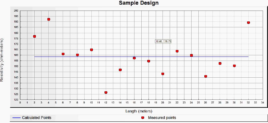
- Resistivity values which are acquired from Wenner-four-pin test results are given in Table 1 A, B, C are different horizontal paths in the region and D is the vertical path in the center of the region.
Table 1 – Wenner test results for uniform soil problem
| a (m) | A | B | C | D | Average |
| 2 | 127 | 209 | 179 | 191 | 176.5 |
| 4 | 138 | 241 | 185 | 204 | 192 |
| 6 | 118 | 236 | 128 | 161 | 160.75 |
| 8 | 120 | 242 | 133 | 145 | 160 |
| 10 | 122 | 242 | 129 | 165 | 164.5 |
| 12 | 129 | 121 | 95 | 160 | 126.25 |
| 14 | 133 | 183 | 130 | 140 | 146.5 |
| 16 | 152 | 184 | 120 | 172 | 157 |
| 18 | 159 | 166 | 148 | – | 154.33 |
| 20 | 151 | 175 | 103 | – | 143 |
| 22 | 169 | 206 | 115 | – | 163.33 |
| 24 | 154 | 222 | 103 | – | 159.67 |
| 26 | 158 | 152 | 112 | – | 140.67 |
| 28 | 156 | 170 | 131 | – | 152.33 |
| 30 | 160 | 199 | 92 | – | 150.33 |
| 32 | 177 | 230 | 160 | – | 189 |
| Total Average: | 158.51 | ||||
Two separate solutions are given here. Solution 1 includes a designed grid in a uniform soil model composed of rods and grid conductors given in Turkish standards. First grounding parameters are observed without overhead line effect (current division factor) on the design.
Then, this effect is considered and parameters are recalculated. The enhancement of the design is observed.
Solution 2 includes the same grid configuration except the soil model. In this case, two layer soil model is used and grounding parameters are observed and compared with Solution 1.
Solution 1
In order to obtain uniform soil model, Wenner-four-pin test results have to be considered. A graph that is composed of average resistivity values obtained from different electrode spacings is drawn to calculate approximate soil resistivity and it is given in Figure 2.
Since all the results close to each other, taking the average value of all results for different electrode spacings can be used to determine the soil resistivity as it is given in Table 1. Uniform soil resistivity value is computed as 158,51 Ω and in Figure 2, this average value is drawn as a line.
Figure 2 – Sample design soil resistivity determination
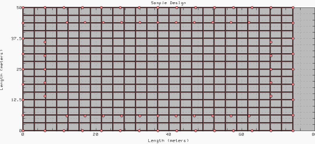
An initial grid configuration is designed by the author and it is given in Figure 3 There are 76 rods in this design and total length of grid conductors used in design is 2508 m. With the given grid configuration, Thapar-Gerez method ground resistance (R) is determined to be 1.33 Ω.
On the other hand, FEM analysis compute ground resistance (R) to be 1.11 Ω for the same grid design.
Figure 3 – Sample grid design
Ground potential rise (GPR=R·IG) of the given grid design is computed by ground resistance (1.11 Ω) and grid current (IG = 20kA). Moreover grid current is calculated by division factor (S f = 1), reduction factor (r = 0.65) and decrement factor (Df = 1.0313). These values are chosen according to national standards and none of them are computed explicitly for this specific problem.
From these calculations, GPR is calculated to be 22973 Volts. Maximum permissible touch potential is calculated as 877 Volts and Figure 4 shows the touch, step and surface potential distributions along the grounded area.
Figure 4 – Potential distributions of sample design
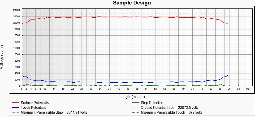
In Figure 4, step potential distribution is always under maximum permissible step potential (2841 Volts). On the other hand, touch potential in the region is not safe because value of touch potential is bigger than maximum permissible touch potential for most of the points.
In Figure 5, touch potential distribution is given in three dimensional view.
Figure 5 – Touch potential distribution of sample design
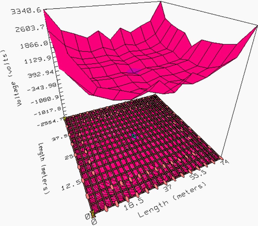
In this figure, all regions are in the danger of high touch potential. Therefore, it can be observed that the design has to be enhanced. For the enhancement of design, division factor is recalculated for this special substation configuration without omitting overhead line impedance.
| Title: | A Handbook for Solving Problematic Cases in AC Substation Grounding Systems – Mustafa Güçlü Aydiner |
| Format: | |
| Size: | 2.0 MB |
| Pages: | 118 |
| Download: | Here 🔗 (Get Premium Membership) | Video Courses | Download Updates |
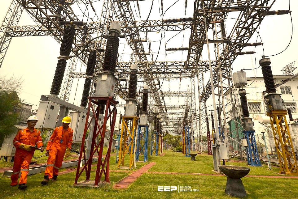
Good Reading – Mechanical Check, Visual Inspection and Electrical Test of the Substation Grounding System
Mechanical Check, Visual Inspection and Electrical Test of the Substation Grounding System (1)
Mechanical Check, Visual Inspection and Electrical Test of the Substation Grounding System (2)

Highest, and very opportunes, considerations about earthing systems in electric power substations !
Good coursed