
Estimated Study Time: 19 minutes
Transformer exciting and inrush currents
If normal voltage is impressed across the primary terminals of a transformer with its secondary open-circuited, a small exciting current flows. This exciting current consists of two components, the loss component and the magnetizing component. The loss component is in phase with the impressed voltage, and its magnitude depends upon the no-load losses of the transformer.
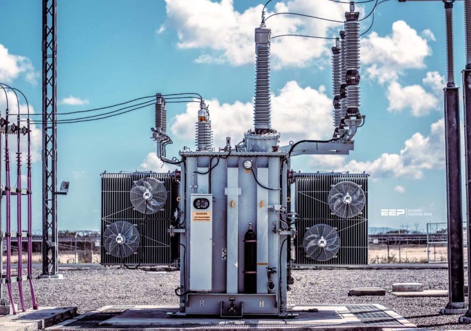 Exciting and inrush currents in transformers that often make protection relays go crazy (photo credit: Andrew George Cowan via Flickr)
The magnetizing component lags the impressed voltage by 90 electrical degrees, and its magnitude depends upon the number of turns in the primary winding, the shape of the transformer saturation curve and the maximum flux density for which the transformer was designed.
A brief discussion of each of these components follows:
- Magnetizing Component of Exciting Current
- Loss Component of Exciting Current
- Total Exciting Current
- Typical Magnitudes of Exciting Current
- Inrush Current
- Determination of Current Inrush
1. Magnetizing Component of Exciting Current
If the secondary of the transformer is open, the transformer can be treated as an iron-core reactor. The differential equation for the circuit consisting of the supply and the transformer can be written as follows:
e = R×i + n1×dΦ/dt
where,
- e = instantaneous value of supply voltage
- i = instantaneous value of current
- R = effective resistance of the winding
- Φ = instantaneous flux threading primary winding
- n1 = primary turns
Normally the resistance, R, and the exciting current, i are small. Consequently the R×i term in the above equation has little effect on the flux in the transformer and can, for the purpose of discussion, be neglected. Under these conditions Equation (1) can be rewritten:
e = n1× dΦ/dt (equation 1)
If the supply voltage is a sine wave voltage,
e = √2 E sin (ωt+λ) (equation 2)
where, E is a rms value of supply voltage, ω = 2πf
Substituting in Equation (1):
√2 E sin (ωt+λ) = n1× dΦ/dt
Solving the above differential equation,
Φ = (− √2 E cos (ωt+λ)) / ωn1 + Φt (equation 3)
Under steady-state conditions this component is equal to zero; the magnitude of Φt is discussed in Section 5.
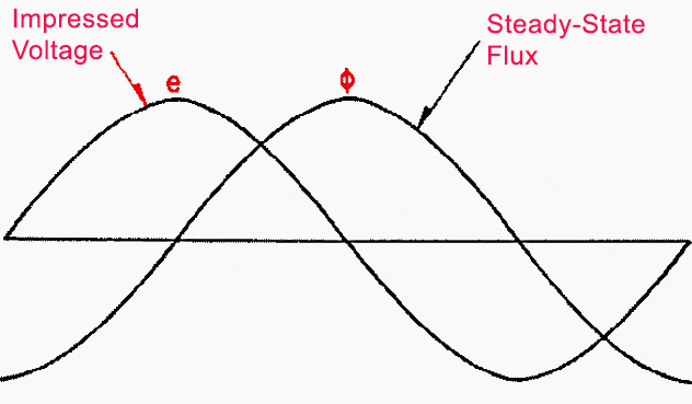
From Equation (3) it can be seen that the normal steady-state flux is a sine wave and lags the sine wave supply voltage by 90 degrees. The supply voltage and the normal flux are plotted in Figure 1 as a function of time.
If there were no appreciable saturation in the magnetic circuit in a transformer, the magnetizing current and the flux would vary in direct proportion, resulting in a sinusoidal magnetizing current wave in phase with the flux. However, the economic design of a power transformer requires that the transformer iron he worked at the curved part of the saturation curve, resulting in appreciable saturation.
In Figure 2(b) are shown the impressed voltage and the flux wave lagging the voltage by 90 degrees. For any flux the corresponding value of current can be found from the B-H curve. Following this procedure the entire current wave can be plotted. The current found in this manner does not consist of magnetizing current alone but includes a loss component required to furnish the hysteresis loss of the core.
However, this component is quite small in comparison to the magnetizing component and has little effect on the maximum value of the total current.
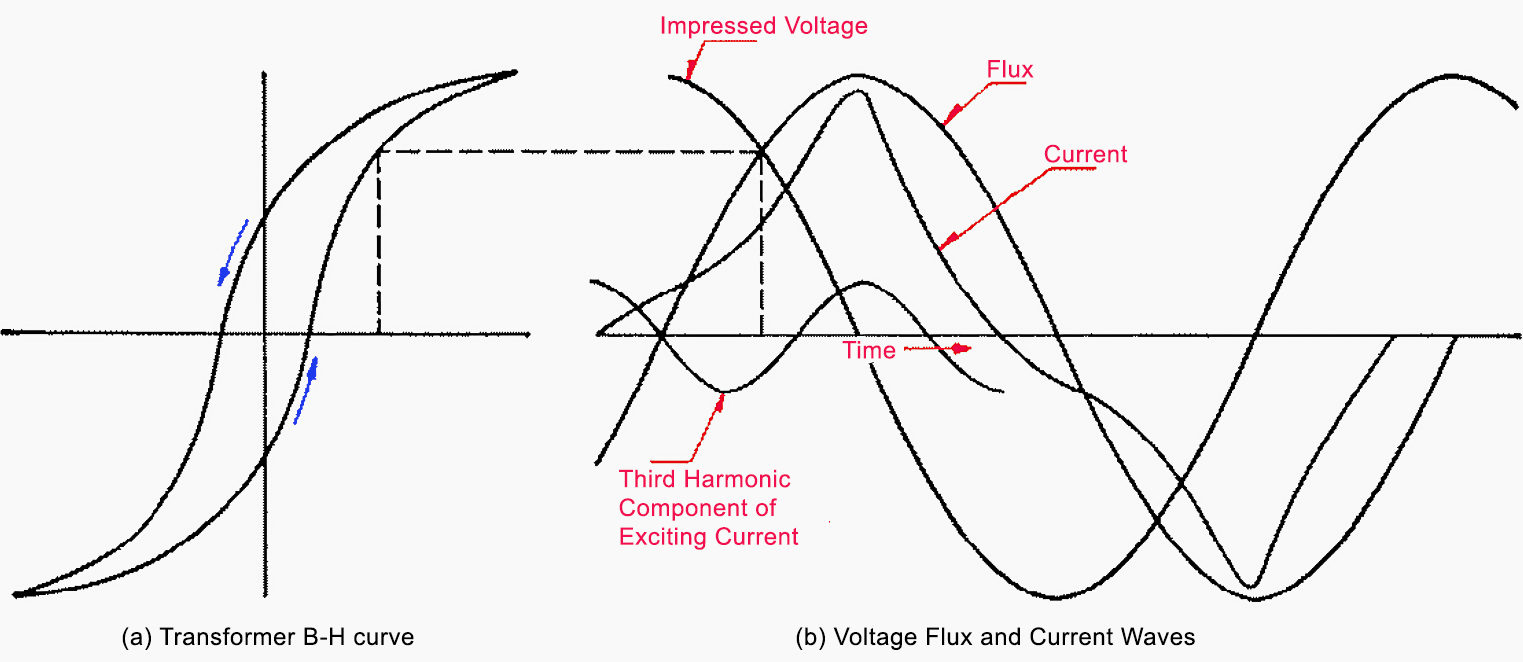
A study of Figure 2 shows that although the flux is a sine wave the current is a distorted wave. An analysis of this current wave shows that it contains odd-harmonic components of appreciable magnitude; the third harmonic component is included in Figure 2.
In a typical case the harmonics may be as follows: 45 percent third, 15 percent fifth, three percent seventh, and smaller percentages of higher frequency. The above components are expressed in percent of the equivalent sine wave value of the total exciting current. These percentages of harmonic currents will not change much with changes in transformer terminal voltage over the usual ranges in terminal voltage.
In Figure 3 are shown the variations in the harmonic content of the exciting current for a particular grade of silicon steel.

2. Loss Component of Exciting Current
The no-load losses of a transformer are the iron losses, a small dielectric loss, and the copper loss caused by the exciting current. Usually only the iron losses, i.e., hysteresis and eddy current losses, are important. These losses depend upon frequency, maximum flux density, and the characteristics of the magnetic circuit. In practice the iron losses are determined from laboratory tests on samples of transformer steel.
However, the formulas given below are useful in showing the qualitative effect of the various factors on loss.
- Iron loss= Wh + We
- Wh = Kh f Bxmax watts per lib
- We = Ke f2t2 B2max watts per lib
Where,
- Wh = hysteresis loss
- We = eddy current loss
- f = frequency
- f = thickness of laminations
- Bmax = maximum flux density
Kh, Ke and x are factors that depend upon the quality of the steel used in the core. In the original derivation of the hysteresis loss formula by Dr. Steinmetz, x was 1.6. For modern steels x may have a value as high as 3.0. The iron loss in a 60-cycle power transformer of modern design is approximately one watt per pound.
Tile ratio of hysteresis loss to eddy current loss will be on the order of 3.0 with silicon steel and 3,6 with oriented steel. These figures should be used as a rough guide only, as they vary considerably with transformer design.
3. Total Exciting Current
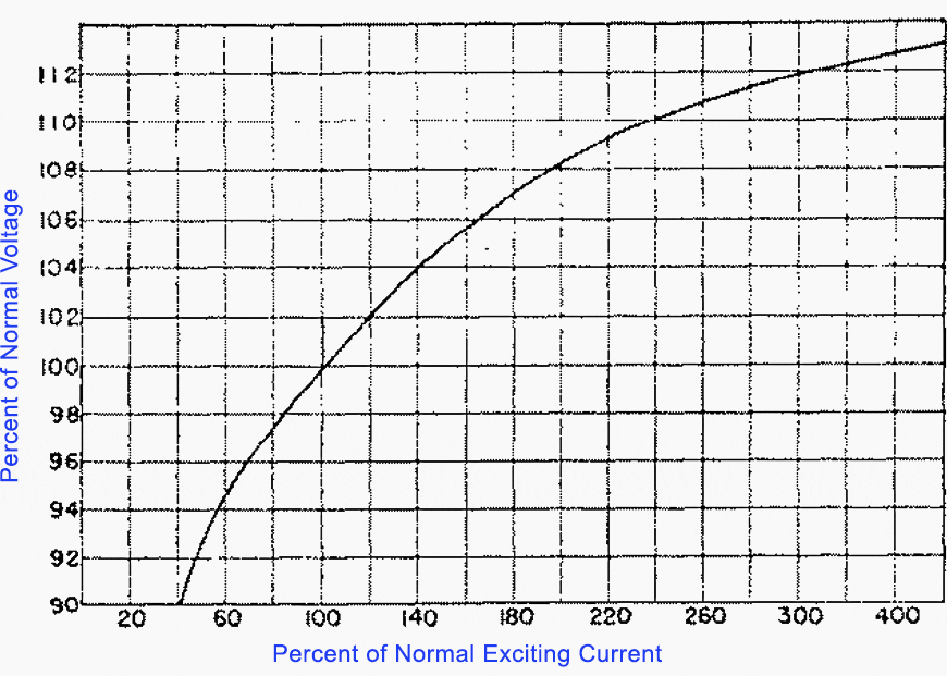
As discussed above, the total exciting current of a transformer includes a magnetizing and a loss component. The economic design of a transformer dictates working the iron at the curved part of the saturation curve at normal voltage; hence any increase in terminal voltage above normal will greatly increase the exciting current.
In Figure 4 the exciting current of a typical transformer is given as a function of the voltage applied to its terminals. The exciting current increases far more rapidly than the terminal voltage.
For example. 108-percent terminal voltage results in 200-percent exciting current.
4. Typical Magnitudes of Exciting Current
The actual magnitudes of exciting currents vary over fairly wide ranges depending upon transformer size, voltage class, etc. In Table 1 are given typical exciting currents for power transformers. The exciting currents vary directly with the voltage rating and inversely with the kVA rating.
Table 1 – Typical exciting current values for single-phase power transformers (in percent of full load current)
| 3-phase kVA | Voltage Class (Full Insulation) | ||||||
| 2.5 kV | 15 kV | 25 kV | 69 kV | 138 kV | 161 kV | 230 kV | |
| 500 | 3.7% | 3.7% | 3.8% | 4.9% | |||
| 1 000 | 3.3% | 3.3% | 3.6% | 4.3% | |||
| 2 500 | 3.1% | 3.2% | 3.8% | ||||
| 5 000 | 2.8% | 3.1% | 2.5% | 4.1% | |||
| 10 000 | 3.0% | 3.1% | 2.4% | 3.6% | 4.0% * | ||
| 25 000 | 2.2% | 2.4% | 3.1% | 3.9% | 3.5% * | ||
| 50 000 | 3.1% | 3.9% | 2.8% * | ||||
* Reduced insulation
The following values should be considered as very approximate for average standard designs and are predicated on prevailing performance characteristics. Test values will as a rule come below these values but a plus or minus variation must be expected depending upon purchaser’s requirements.
Should closer estimating data be required, the matter should be referred to the proper manufacturer’s design engineers.
5. Inrush Current
When a transformer is first energized, a transient exciting current flows to bridge the gap between the conditions existing before the transformer is energized and the conditions dictated by steady-state requirements.
For any given transformer this transient current depends upon the magnitude of the supply voltage at the instant the transformer is energized, the residual flux in the core, and the impedance of the supply circuit.
In studying the phenomena that occur when a transformer is energized it is more satisfactory to determine the flux in the magnetic circuit first and then derive the current from the flux. This procedure is preferable because the flux does not depart much from a sine wave even though the current wave is usually distorted.
The total flux in a transformer core is equal to the nor-mal steady-state flux plus a transient component of flux, as shown in Equation (3). This relation can be used to determine the transient flux in the core of a transformer immediately a/2 after the transformer is energized.
As √2E/ωn1 represents the tons crest of the normal steady-state flux, Equation (3) can be rewritten as:
Φ = − Φm cos (ωt+λ) + Φt (Equation 4)
where Φm = √2E/ωn1
at t = 0 and Φ0 = − Φm cos λ + Φt0
where,
- Φ0 = transformer residual flux
- − Φm cos λ = steady-state flux at t = 0
- Φt0 = initial transient flux
Assume that a transformer having zero residual flux is energized when the supply voltage is at a positive maximum. For these conditions Φ0 and cos λ are both equal to zero so Φt0 also equal to zero. The transformer flux therefore starts out under normal conditions and there would be no transient.
However, if a transformer having zero residual is energized at zero supply voltage the following conditions exist:
λ = 0
− Φm cos λ = − Φm
Φ0 = 0
Φt0 = Φm
Substituting in Equation (4): Φ = − Φm cos (ωt) + Φm (Equation 5)
The flux wave represented by Equation (5) is plotted in Figure 5(a). The total flux wave consists of a sinusoidal flux wave plus a DC flux wave and reaches a crest equal to twice the normal maximum flux.
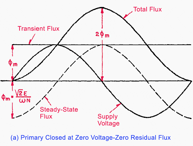
In this figure the transient flux has been assumed to have no decrement; if loss is considered the transient flux decreases with time and the crest value of the total flux is less than shown.
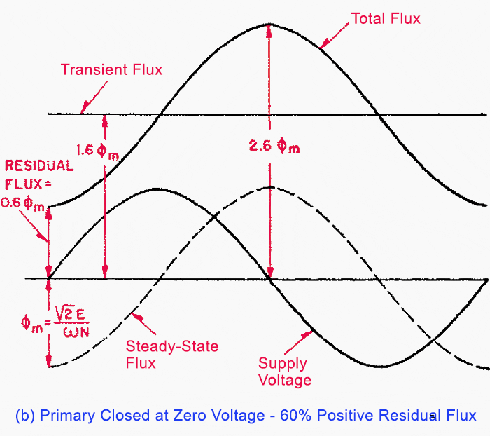
In Figure 5(b) similar waves have been plotted for a transformer having 60 percent positive residual flux and energized at zero supply voltage. Sixty percent residual flux has been assumed for illustration only. Flux waves for any other initial conditions can be calculated in a similar manner using Equation (4).
6. Determination of Current Inrush
After the flux variation has been determined by the method described, the current wave can be obtained graphically as shown in Figure 6. In the case illustrated it was assumed that a transformer having zero residual flux was energized at zero supply voltage; the flux there-fore is equal to twice normal crest flux. For any flux the corresponding current can be obtained from the transformer B-H curve.
In the above discussion loss has been neglected in order to simplify the problem. Loss is important in an actual transformer because it decreases the maximum inrush cur-rent and reduces the exciting current to normal after a period of time.

The losses that are effective are the resistance loss of the supply circuit and the resistance and stray loosed in the transformer.
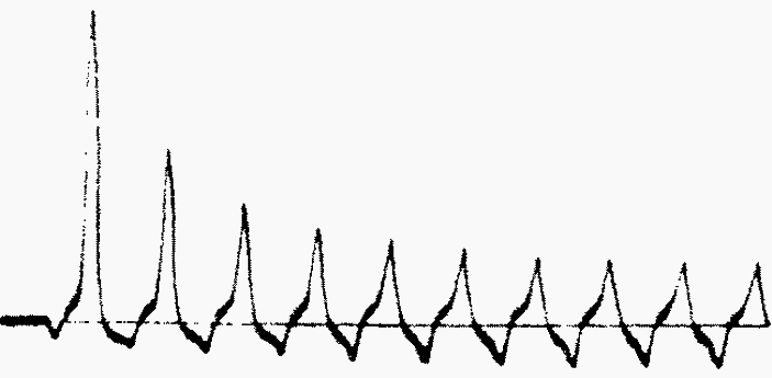
Figure 7 is an oscillogram of a typical exciting-current inrush for a single-phase transformer energized at the zero point on the supply voltage wave. The transient has a rapid decrement during the first few cycles and decays more slowly thereafter. The damping coefficient, R/L for this circuit is not constant because of the variation of the transformer inductance with saturation.
During the first few current peaks, the degree of saturation of the iron is high, making L low. The inductance of the transformer increases as the saturation decreases, and hence the damping factor becomes smaller as the current decays.
7. Estimating Inrush Currents
The calculation of the inrush current to a power transformer requires considerable detailed transformer design information not readily available to the application engineer. For this reason reference should be made to the manufacturer in those few cases where a reasonably accurate estimate is required.
An order of magnitude of inrush currents to single-phase, 60-cycle transformers can be obtained from the data in Table 2. The values given are based on the transformer being energized from the high-voltage side at the instant the supply voltage passes through zero. Energizing a core-form transformer from the low-voltage side may result in inrush currents approaching twice the values in the table.
Table 2 – Approximate inrush currents to 60-cycle power transformers energized from the high-voltage side
| Transformer Rating kVA | Core Form | Shell Form |
| 2 000 | 5 – 8 | |
| 10 000 | 4 – 7 | 2.5 – 5 |
| 20 000 | 2.0 – 4 |
The per unit inrush current to a shell-form transformer is approximately the same on the high- and low-voltage sides. The inrush currents in Table 2 are based on energizing a transformer from a zero-reactance source.
When it is desired to give some weight to source reactance, the inrush current may be estimated from the relation:
I = I0 / (1+I0X)
where
- Io = Inrush current neglecting supply reactance in per unit of rated transformer current
- X = Effective supply reactance in per unit on the transformer kva base.
Source: T&D book by ABB
Related electrical guides & articles


Edvard Csanyi
Hi, I'm an electrical engineer, programmer and founder of EEP - Electrical Engineering Portal. I worked twelve years at Schneider Electric in the position of technical support for low- and medium-voltage projects and the design of busbar trunking systems.I'm highly specialized in the design of LV/MV switchgear and low-voltage, high-power busbar trunking (<6300A) in substations, commercial buildings and industry facilities. I'm also a professional in AutoCAD programming.
Profile: Edvard Csanyi

Thank you for these helpful explanations. I just couldn’t understand the difference between the excitation current and the inrush current.
Could you please tell explain what is the difference between them?
Thanks
Excellent job. Very interesting. Thank you.
Is it possible that power fuse @ 175 A with parallel VCB, VCB-1 has connected transformer of 2 MVA, 2 MVA, 3 MVA, & 3.5 MVA while VCB-2 has connected Transformer of 2 MVA. It was approved by Utility Company, There are two incident for different transformer with the same rating @ 2 MVA, A huge fault has been recorded the primary side of transformer at around 536Amps, causing burn out at the primary winding of transformer… I Appreciate your comment on this matter, Thank you.
Thanks you for the good information
I need information about power systems protection.
Discussion on inrush current&exciting current is very clear to understand &
Mathematical deduction of differential equation is helpful for engineers at any stage.
Dhaka,Bangladesh.
It’s an informative lesson.thaks for sharing.really I like it very much