
Estimated Study Time: 42 minutes
Where’s the energy going?
Nowadays, the enormous energy consumption worldwide has taken a downturn due to the hiking energy prices. Whether it’s gas, oil, or coal, the rising costs forced many facilities worldwide to cut their energy expenses. This is a good moment to start questioning facility power consumption and find where the energy is going, because for many businesses, increasing of energy bills and doing nothing about it usually means closing.
 How should facilities optimize their power consumption due to the hiking energy prices?
An important initial step in evaluating energy saving opportunities is to estimate The contribution to peak billing demand, and the amount of energy consumption. Of each major load or process within the facility being evaluated.
Generally, the facility energy profile helps to focus the energy optimization efforts on those processes or loads that have the most savings potential. This profile also may identify batch processes or discretionary loads that may be scheduled at times of low demand for the rest of the facility, or during times of off-peak utility prices.
This fact would suggest that the meter measuring the power consumption of a feeder serving the building’s centrifugal water chillers.
An example of the facility energy profile looks like this:
- Chillers: 33% (highest demand)
- HVAC: 10%
- Chilled Water Pumps: 9%
- Production Equipment: 9%
- Compressed Air: 8%
- Lighting Systems: 8%
- Packaging Lines: 8%
- Miscellaneous: 6%
- Utility Systems: 3%
- Cooling Tower Fans: 3%
- Condenser Water Pumps: 3%
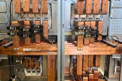
Actual power monitoring data from existing circuit monitors measuring the power consumption of individual feeders is the best basis for establishing the Facility Energy Profile
Figure 1 – Power monitoring of existing circuits
Let’s start the discussion with defining demand analysis techniques, demand controls systems, optimizing the demand savings associated with generator operation, lighting control and later with optimizing electric motors, VSDs, compressed air, an so on.
- Demand analysis techniques
- Demand control
- Peak shaving with on-site generators
- Lighting control
- Electric motors
- Variable-speed drives (VSDs)
- Compressed air
- Centrifugal water chillers
- Heating, ventilating, and air conditioning systems
- Energy survey checklist
1. Demand analysis techniques
Demand analysis is the methodology used to determine if there are opportunities for a given facility to reduce peak demand charges. Demand analysis involves manipulation of historical demand interval data to determine:
- Which major processes or loads are operating at times of highest demand;
- How “steep” or “flat” the facility’s load profile appears; and
- What times of day these peaks are occurring.
The demand sort is produced by rearranging individual integrated demand readings for a given billing period. Meters record demand readings chronologically, 3000 or so readings for a 30-day billing period at 15-minute demand intervals; the demand sort utilizes a software tool to distribute the readings from highest to lowest, so that times and values of peak usage are easily analyzed.
Figure 2 – Energy demand statistics
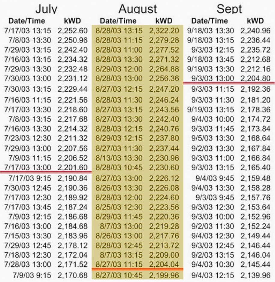
Figure 4 shows the demand sort table facilitates demand analysis by depicting the number of intervals (or hours) during which the plant’s peak electrical demand exceeded certain levels.
Figure 3 – The demand sort table
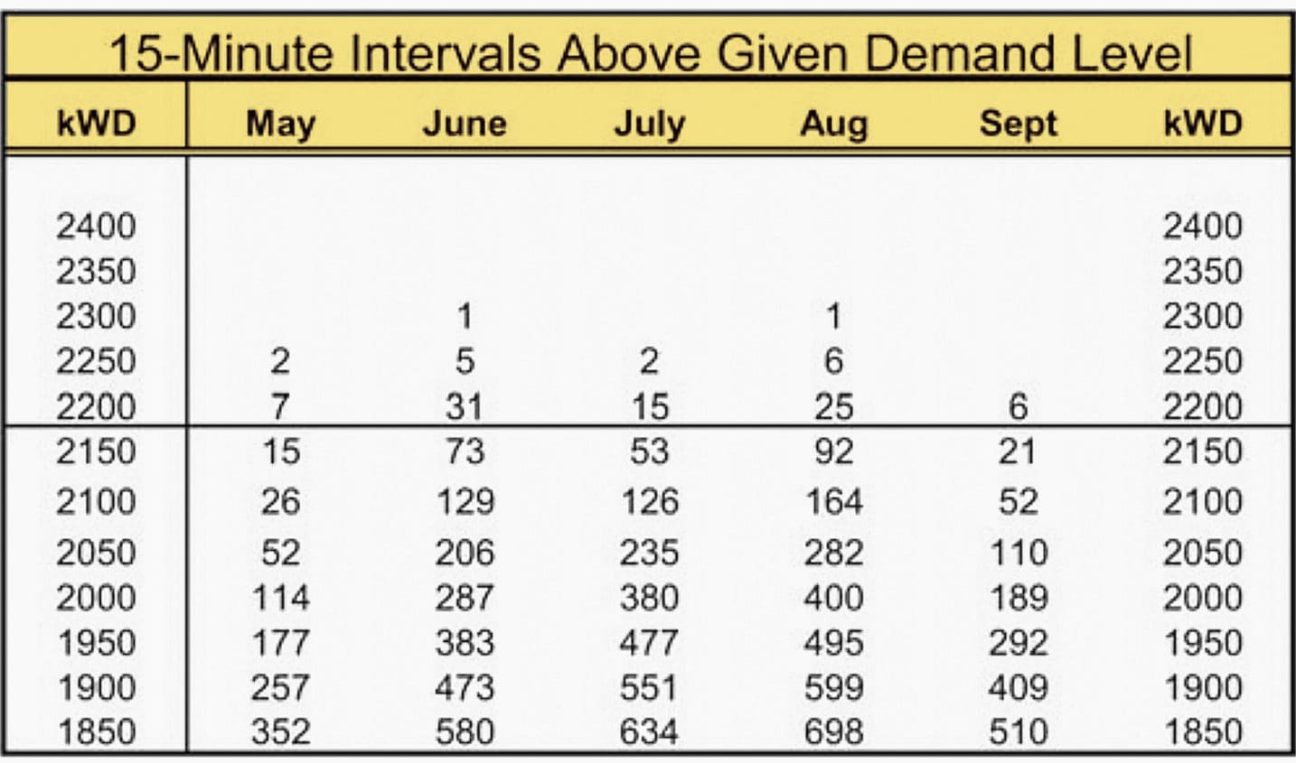
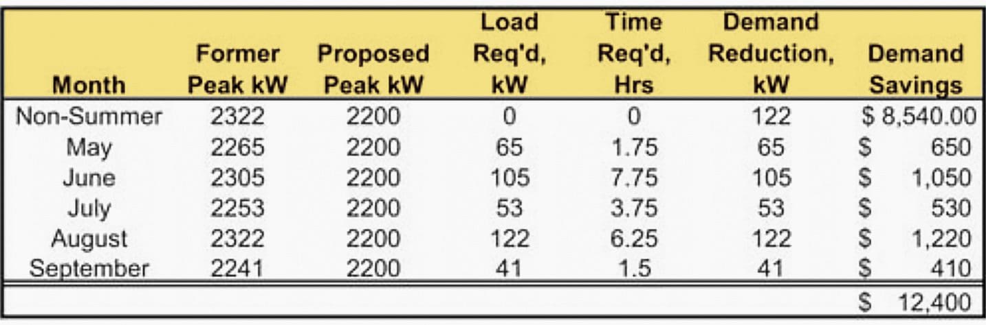
Using the demand sort table, the engineer is able to determine that a reduction in peak demand to 2200 kW at this example facility would have required a demand reduction of 122 kW for 25 15-minute intervals, or 6.25 hours, in August of the sample year.
Figure 4 – An example of reduction in peak demand to 2200 kW
Facility Peak-Day load profiles from actual power monitoring data can show consistency, or, as in this case, a single-day aberration in peak demand that set the demand minimum billing level (ratchet) for the remainder of the year.
Figure 5 – Facility Peak-Day load profile
Go back to the Contents Table ↑
2. Demand control
Demand controls systems are available that perform the following basic functions:
- Measure power consumption (demand) in real time
- Predict demand level based on rate of instantaneous usage
- Compare predicted value to target setpoint
- Transmit signals to pre-determined equipment to turn off or curtail power usage if demand is predicted to exceed target kW
These demand controls systems are intended to reduce peak demand for a facility to some predetermined level. The design engineer’s foremost demand control system challenge is to identify loads in the facility that can be controlled effectively.
Ideal load candidates includes those machines or processes that are currently contributing to the facility’s load at peak times, and whose function can be delayed or curtailed at times of peak. Most facilities lack equipment or processes that fit this ideal description, despite the numerous machines and processes that may be operating at peak times.
In fact, successful demand control is usually the exception rather than the rule!
One common candidate for the demand control system is the air conditioning system. Buildings equipped with multiple packaged direct-expansion air conditioning systems are typical targets of demand control sales efforts. Unfortunately, demand control of air conditioning compressors usually leads to loss of temperature or humidity control within the conditioned space, or lack of demand savings.
Secondly, basic thermodynamic principles of moist air and vapor-compression refrigeration systems require compressor power consumption to reduce air temperature and condense moisture. This process is controlled by thermostats and humidistats within the facility. When cooling or dehumidification is removed or reduced at times when these devices are “calling for” them, temperature and humidity will rise in the conditioned space.
So, if not air conditioning equipment, what loads have been successful demand control candidates?
An electrolysis process providing chemicals for a paper mill was able to reduce peak demand and flatten the demand profile for the overall facility. A battery-charging system for forklift vehicles in an automotive facility was capable of producing real demand savings during peak times.
Finally, a large induction furnace melting scrap metal proved to be an effective candidate for the rolling mill at a steel plant.
Figure below shows how chilled water supply and return temperatures increase over the course of a day due to demand control of inlet guide vanes on a centrifugal water chiller. Space conditions could not be maintained as a result of the demand control.
Figure 6 – Chilled water supply and return temperatures increase
Go back to the Contents Table ↑
3. Peak shaving with on-site generators
How, the engineer might ask, can a facility save money by burning fossil fuel in an onsite generator at a unit cost of 12 ¢/kWh, when the average unit cost of utility purchased power is 8 ¢/kWh? Very carefully, is the expected – and accurate – response.
The key to economical peak shaving is to understand and optimize the demand savings associated with generator operation. That is, the onsite generator must be operated the absolute minimum time necessary to reduce peak demand the maximum amount. Because the overall average unit price of electricity is not necessarily equivalent to the effective price of electricity at the plant’s peak.
For the facility with a sharp demand peak, when the peak for the month is set in a few hours or less and the remainder of the time demand is low, peak-shaving at 12 ¢/kWh can be preferable to paying 20 ¢/kWh.
Go back to the Contents Table ↑
3.1 Costs of generated power
Onsite generators typically utilize natural gas, wood, fuel oil, or steam derived from a fossil fuel or as a part of a production process. Unit fuel costs for fossil fuels are usually calculated based on the fuel’s heating value, an estimated efficiency of the generator system, and the fuel cost.
Cost/kWh = fuel price/gal × 3413/HV/efficiency
In this equation, HV is the heating value of fuel oil in BTU/gal, and 3413 is the conversion from BTU to kWh. Internal combustion diesel generators typically range in efficiency from 25-30%.
For a typical example, #2 fuel oil may be burned in an IC engine. For a fuel-oil price of $2.00/gal, and a generator efficiency of 25%, the fuel cost/kWh is:
- Cost/kWh = $2.00 × 3413/108,000 BTU/gal/0.25
- Cost/kWh = 25 ¢/kWh
Obviously, peak-shaving is much less attractive at a fuel cost of $2.00/gal, unless required generator operation can be predicted accurately and electricity charges are comparably high as well.
Go back to the Contents Table ↑
3.2 Utility rates affecting peak-shaving generation
Electric utility rates must be analyzed carefully prior to implementing peak shaving or cogeneration opportunities. Some utilities have special interconnection and protective relaying requirements to ensure that onsite generation does not pose a safety hazard for utility workers.
In addition, many utility rate schedules impose standby charges for onsite generation.
Facilities with onsite generation may be able to operate this equipment to reduce purchased power requirements during periods of high demand, or high utility prices.
Figure 7 – Reducing purchased power requirements with onsite generation
Figure below shows how savings or losses associated with operation of peak-shaving generators are dependent on fuel prices, on-peak electricity prices, the amount of time the generator has to operate for a given peak-reduction target, and, most importantly, the accuracy with which plant personnel can predict these variables.
Figure 8 – Savings or losses are associated with operation of peak-shaving generators
Electricity generation and peak shaving can also be accomplished with steam cogeneration systems typical of paper mills, refineries, and other large industrial processes.
Figure 9 – Steam cogeneration system diagram
Go back to the Contents Table ↑
4. Lighting control
Lighting systems in industrial facilities can represent an attractive savings opportunity, especially if lighting systems have not been upgraded or maintained in the past ten years. The most cost-effective approach for lighting energy savings is to address the following three issues, in order:
- Turn off lights during times when they are not needed
- Reduce light levels to match the requirements for the tasks being performed in the area
- Replace less efficient lamps, ballasts, or fixtures with more efficient sources
The second priority in lighting conservation involves light level reductions. The Illuminating Engineering Society of North America (www.iesna.org) has established recommended light levels for different types of work tasks and area usage types.
Light output of a fixture is usually published in lumens. Many manufacturers of lamps and lighting systems offer software tools to aid in designing new systems, or in evaluating changes to existing systems.
Suggested Course – Ultimate Course To Electrical Drawings Design Using AutoCAD, DiaLUX & ETAP
Ultimate Course To Electrical Drawings Design Using AutoCAD, DiaLUX and ETAP Software
Go back to the Contents Table ↑
4.1 Some lighting essentials
4.1.1 Lighting controls work better than people
While “turn-off-the-light” programs have been widely utilized in all types of facilities, sophisticated lighting control systems have proven to be much more cost-effective. Certainly, it’s cheaper to have a worker turn off a light, but workers forget, workers may not have access to circuit breakers controlling large banks of industrial lighting fixtures, those same circuit breakers are not designed for daily operation as light switches, and so on.
Lighting system controls that utilize microprocessors and specially-designed remote-operated circuit breakers are much more effective. These devices can be programmed to accommodate complicated shift configurations, including nights, weekends, and holidays. They also include simple over-ride features for temporary or unusual work schedules.
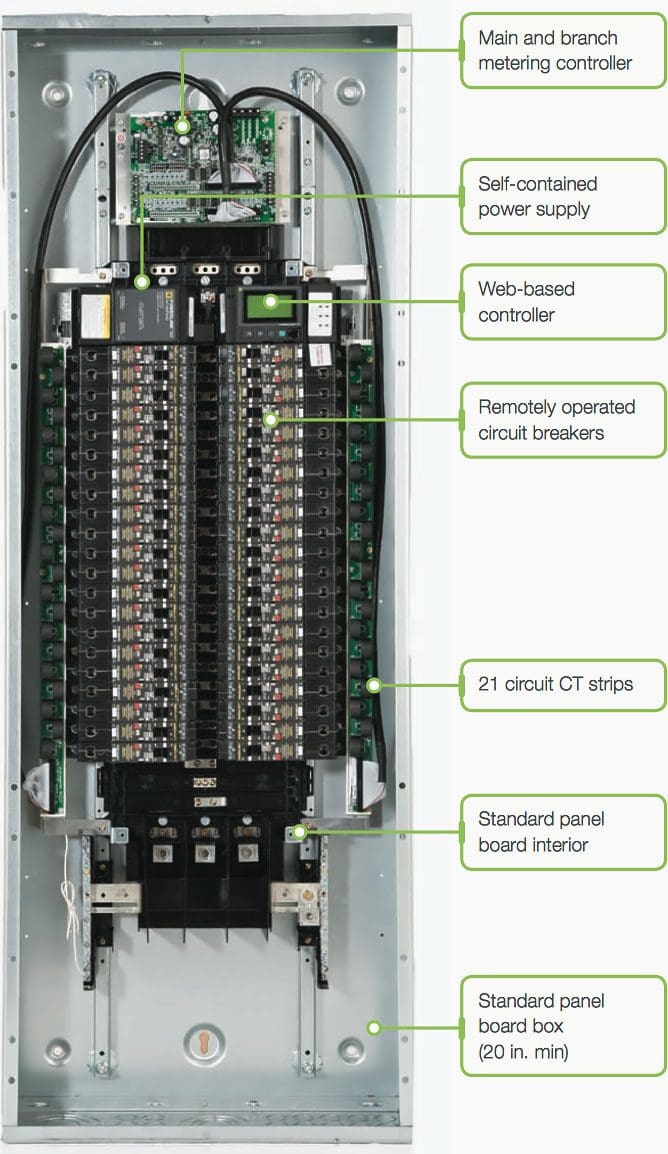
For example, Powerlink MVP Intelligent lighting panel (by Schneider Electric) utilizes patented technology to control lighting circuits, and offers Transparent Ready web-based monitoring and control
Figure 10 – Powerlink MVP Intelligent lighting panel (by Schneider Electric)
Go back to the Contents Table ↑
4.1.2 Light levels decline with age of the lighting system
Several factors contribute to this decline. Lamps, including fluorescent and high-intensity discharge sources like high-pressure sodium and metal halide, experience Lamp Lumen Depreciation (LLD). The LLD is typically less than 1.0, indicating that average lamp light output at some point in the future is less than light output of a new lamp.
Light levels are also adversely affect by dirt and the accumulation of dust on the light fixture. Luminaire Dirt Depreciation (LDD), also a factor less than 1.0, is a function of the type of light fixture as well as the environment in which the fixture operates.
Ballast Factor, or BF, is yet another commonly used factor. BF is also a published value that is a function of the type of ballast used to control the arc characteristics of fluorescent and HID lighting systems.
The designer usually applies these factors to the rated light level output of a lighting system, in order to estimate the number of fixtures required to provide the desired light level – not at initial installation, rather at some designated point in the future. For example,
# fixtures = total required lumens/initial lumens/fixture/(LLD * LDD * BF)
Suggested Course – Electrical Designing and Drafting Course
Go back to the Contents Table ↑
4.1.3 Lighting designers need to know the facility’s lamp replacement practices
Manufacturers publish the “rated life” expectancy of a given lamp. This value, usually given in thousands of hours, is not a guarantee that every lamp will extinguish at the same rated-life time. In fact, the “rated life” is a statistical value indicating the point at which half of the lamps of a representative sample will burn out. Some lamps will fail well shy of the rated life; others may last beyond the rated life.
The facility’s lamp replacement practices usually fall into one of two categories:
- Replace individual lamps as they fail (“spot replacement”)
- Replace all lamps at a predetermined point in time, even though many of those lamps are still burning (“group replacement”)
Group replacement runs counter to common sense for most people – if it ain’t broke, don’t fix it. That’s why spot replacement is the most common practice by far. There is, however, a sound reason for considering the group-replacement strategy: Economics.
Fewer light fixtures means lower energy costs attributable to lighting, and less heat for the building’s air conditioning system. Labor costs have also been shown to be lower for group replacement as compared to spot replacement. Group replacement can be scheduled to occur during unoccupied times; set up and take down costs are reduced; the cost per lamp itself can be lower with large-quantity purchases.
Suggested Course – AC Distribution Panel Drawings: Single-Line Diagrams, Wirings & Interlocking Schematics
Learn AC Distribution Panel Drawings: Single-Line Diagrams, Wirings, and Interlocking Schematics
Go back to the Contents Table ↑
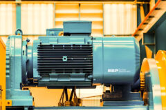
5. Electric motors
Three-phase squirrel-cage induction motors comprise a considerable percentage of the electrical load in the United States. Design, operation, and maintenance of these machines is well described in other references; this document focuses on their energy efficiency aspects.
Induction motors typically range in full load efficiency from about 87% to 94%. This efficiency is very difficult to measure accurately in the field, requiring a dynamometer and other specialized equipment. Fortunately, energy saving projects associated with electric motors do not require actual efficiency of a given motor to be established.
One of the foremost opportunities for energy savings is to implement a program of replacing – rather than rewinding – induction motors at failure. Rewinding a damaged induction motor is a common practice in industry, but studies have proven that rewinding an induction motor drops its efficiency by a couple percentage points.
The incremental cost of replacing this failed motor with an energy-efficient motor, however, is only $430. This amount assumes considers the rewound cost, and the labor necessary to perform the motor change-out, as sunk costs.
The annual energy savings associated with replacing the failed motor with an energy-efficient model, at a new efficiency of 92.9%, is approximately $510. The simple payback for the replacement, therefore, is less than one year.
Energy-efficient motor programs are applicable to any AC motor installations utilizing NEMA Design B induction motors. Since the programs are based on replacement at failure, the full savings potential is realized after three years or more.
Table 1 – Published efficiencies of typical rewound, standard, and energy-efficient three-phase induction motors.
| HP | Rewound Efficiency | Standard Efficiency | Energy Efficient Efficiency |
| 1 | 69.7% | 70.7% | 82.6% |
| 2 | 79.5% | 80.5% | 83.4% |
| 3 | 79.4% | 80.4% | 86.6% |
| 5 | 81.4% | 82.4% | 88.3% |
| 8 | 83.1% | 84.1% | 90.0% |
| 10 | 85.1% | 86.1% | 91.1% |
| 15 | 85.5% | 86.5% | 92.0% |
| 20 | 87.3% | 88.3% | 92.9% |
| 25 | 88.0% | 89.0% | 93.5% |
| 30 | 88.1% | 89.1% | 93.7% |
| 40 | 88.7% | 89.7% | 94.2% |
| 50 | 90.0% | 91.0% | 94.4% |
| 60 | 89.9% | 90.9% | 94.7% |
| 75 | 90.4% | 91.4% | 94.9% |
| 100 | 90.4% | 91.4% | 95.4% |
| 125 | 90.6% | 91.6% | 95.3% |
| 150 | 91.5% | 92.5% | 95.7% |
Figure 11 – Electric motors are efficient machines, even at partial load
Figure 12 – But power factor drops off sharply at half load
Suggested Course – The Essentials of Rotating Electrical Machines: AC & DC Electric Motors and Generators
The Essentials of Rotating Electrical Machines: AC & DC Electric Motors and Generators
Go back to the Contents Table ↑
6. Variable-speed drives (VSDs)
There are many devices used to provide AC motor control – starting, stopping, changing speed, varying torque, providing protection from voltage and current anomalies. This section will focus, however, on variable-frequency control devices designed to reduce energy consumption and improve operation of three-phase AC induction motors.
Table 2 – Four major categories of AC motor loads
| Load Type | Typical Examples |
| Variable torque | Centrifugal pumps and fans |
| Constant torque | Reciprocating pumps, conveyors, hoists |
| Constant horsepower | Grinders |
| Impact | Punch press |
Energy-saving opportunities commonly focus on the variable-torque category, because the energy saving potential is large even with small changes in pump or fan speed control. This opportunity is driven by the power and speed characteristics of the variable-torque load. The capacity of a pump or fan is directly proportional to the speed. A change in speed of 10% yields a change in pump gpm or fan CFM of 10%.
Brake horsepower, however, is proportionally to the cube of the speed, meaning that a 10% reduction in pump or fan speed can yield a 27% reduction in power consumption.
Since most pumps and fans are driven by fixed-speed electric motors, where speed of the driven load is determined by the number of motor poles, AC frequency, and motor slip, varying the speed of a motor requires an external device. This external device is commonly referred to as an adjustable-speed drive, variable-frequency drive, inverter, vector drive, or adjustable-frequency controller.
Figure 13 – Variable-torque loads, such as centrifugal pumps and fans, exhibit a cubic relationship between brake horsepower and speed
Suggested Reading – Inside Variable Frequency Drive (VFD) Panel
Inside Variable Frequency Drive (VFD) Panel: Configuration, Schematics and Troubleshooting
Go back to the Contents Table ↑
7. Compressed air
Compressed air systems can consume a significant amount of electric energy in an industrial facility. Many textile, automotive, chemical, and petroleum facilities operate large, multi-stage air compressors driven by electric motors representing hundreds, thousands, or even ten-thousands of horsepower in capacity.
One chemical plant providing raw materials for synthetic textile manufacturing operated one 22,000 hp, and two 8,000 hp compressors in a portion of its process. While the 22,000 hp compressor is rare, significant energy reduction opportunities associated with compressed are available.
Power consumption of a typical air compressor is a function of the air volume required (V), the inlet air temperature (Tin), and the required pressure rise (Pout/Pin)
These opportunities may include:
7.1 Reduce outlet pressure
Compressor discharge pressure in some facilities is set too high. Since the pressure rise across a compressor is a key factor in its power consumption, reducing outlet pressure can offer significant savings. Some reasons for excessive pressure may be straightforward; eg, production equipment with lower requirements has replaced older machines without a corresponding reduction in compressed air setpoint.
Other reasons may be more complex; eg, piping system losses or leaks may force higher setpoints at the compressors in order to provide adequate air pressure at production equipment.
7.2 Reduce air volume (CFM) requirements
Compressed air leaks usually offer the most attractive opportunity for reducing compressed air volume. Some facilities have ignored leaks to the point that one compressor is effectively operating 24/7 simply to serve air leaks.
Suggested Reading – Energy-efficiency opportunities in compressed air systems
Eleven energy-efficiency improvement opportunities in compressed air systems
7.3 Reduce inlet temperature
Warm air is less dense than cold air. As the compressed air work equation above indicates, reducing inlet air temperature can reduce the work associated with a compressor. The usual method of reducing air temperature is to provide outside air intakes for the compressor, rather than allowing the compressor to utilize air from a hot equipment room.
7.4 Increase inlet pressure
It’s common to assume that inlet pressure to a compressor is fixed at atmospheric pressure, but this is a misconception. Air compressor inlet systems, especially air filters, need to be kept clean and free of obstructions. Pressure drop across dirty or blocked intakes serves to reduce the pressure at the compressor and increase power consumption.
Multi-stage air compressors, equipped with inter- and after-coolers to optimize efficiency and provide heat recovery, are common in industrial facilities.
Figure 14 – Multi-stage air compressors, equipped with inter- and after-coolers
Go back to the Contents Table ↑
8. Centrifugal water chillers
Figure 15 – Centrifugal water chillers in Dubai World Trade Center chiller plant
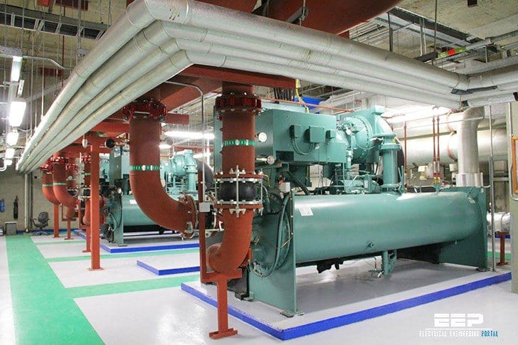
Large commercial and industrial electrical loads are largely made up of centrifugal water chillers. Because of their efficiency, these machines typically produce cooling effects that are two to three times greater than the energy input needed. In the 1980s, centrifugal water systems were the subject of CFC legislation, which led to the replacement or refurbishment of many of these devices. But there are still chances for chiller optimization.
One opportunity is to alter the operational plan for numerous chillers that share a chilled water header. These machines are typically staged so that none are loaded above 80% of their rated capacity. This tactic evolved as a result of the machines’ part-load efficiencies, which tended to produce a U-shaped efficiency curve.
The curve showed that between 60% and 80% of full load was where efficiency was at its highest.
The typical chiller efficiency curve is shaped like an u, with the peak efficiency occurring between 60% and 80% of full load. However, at full load, chillers serving industrial loads have their highest measured efficiency.
Figure 16 – Typical chiller efficiency curve
Figure 17 – Operating three chillers at partial loads is less efficient that operating two chillers at or near their rated capacity
Other successful strategies for chiller optimization include:
Optimization #1 – Chilled water reset
In order to adapt this strategy to the needs of the cooling load, the chilled water supply temperature setpoint must be raised. An automatic chiller controller’s control routines frequently include reset as a step. Resetting a compressor with chilled water can cut power usage by 1.5% to 2% per degree.
Optimization #2 – Reduce condenser water temperature
Similar to raising the chilled water setpoint, reducing the condenser water temperature serves to reduce the compressor power requirements. Condenser water temperature reduction of one degree can reduce compressor power consumption by 0.5%-1%.
Optimization #3 – Monitor and maintain chiller approach temperatures
Chiller condensers and evaporators are shell-and-tube heat exchangers that require periodic maintenance to maintain optimum heat transfer characteristics.
Annual average readings of condenser approach temperature (difference in temperature between condenser water and refrigerant in shell-and-tube heat exchanger) gradually crept up from the initial design value of 6 F to nearly 15 F over three years.
Figure 18 – Annual average readings of condenser approach temperature
Figure 19 – Increase in condenser tube fouling can have a significant adverse effect on compressor power consumption
Go back to the Contents Table ↑
9. Heating, ventilating, and air conditioning systems
HVAC systems should be the focus of a targeted energy study, with similar objectives as the lighting analysis:
- Turn off unnecessary HVAC equipment during unoccupied times
- Match HVAC operation, including temperature and humidity, to minimum occupancy requirements
- Replace inefficient HVAC systems and equipment with energy-saving alternatives
Go back to the Contents Table ↑
10. Energy survey checklist
10.1 Lighting
Table 3 – Checklist and optimization proposal for lighting
| No. | Checklist | Optimization proposal |
| 1 | Lighting operating more hours than needed? | Reduce operating hours with lighting control system. |
| 2 | Areas over lit for task performed? | Reduce light levels by disconnecting or replacing lamps or fixtures. |
| 3 | Incandescent or quartz lamps operating more than 2,000 hours per year? | Convert to LED or other energy efficient source. |
| 4 | Mercury vapor lamps. | Convert to energy saving LED, fluorescent, metal halide, or high-pressure sodium. |
| 5 | Fluorescent at 18-feet or higher mounting heights. | Convert to high pressure sodium or LED. |
| 6 | VHO fluorescent fixtures. | Convert to energy saving LED, fluorescent, metal halide, or high pressure sodium. |
| 7 | Standard fluorescent ballasts. | Replace with energy savings electronic ballasts at failure. |
10.2 Induction motors
Table 4 – Checklist and optimization proposal for induction motors
| No. | Checklist | Optimization proposal |
| 1 | Motors operating 75%+ full load, more than 6,000 hours per year. | Replace with energy efficient motors at failure. |
| 2 | Standard V-belts on pumps or fans. | Convert to cog V-belts. |
| 3 | Fans or pumps that are throttled with dampers or control valves. | Consider variable speed drives. |
10.3 Demand management
Table 5 – Checklist and optimization proposal for demand management
| No. | Checklist | Optimization proposal |
| 1 | Sharp demand peaks of short duration (low load factor)? | Identify loads to shed or reschedule to off-peak. |
| 2 | Batch processes? | Shift to off-peak. |
| 3 | Consider Time-of-Use savings opportunities. | |
10.4 Exhaust, ventilation, and pneumatic conveying
Table 6 – Checklist and optimization proposal for exhaust, ventilation & pneumatic conveying
| No. | Checklist | Optimization proposal |
| 1 | Transport velocities or exhaust flows higher than minimum required? | Consider changing belts and sheaves to reduce air velocity. |
| 2 | Consider variable speed or inlet vane control. | |
| 3 | Consider exhaust air heat recovery. | |
| 4 | Make-up air properly provided for all exhaust? | |
| 5 | Fume hoods designed to minimize exhaust? | |
| 6 | Properly designed stack heads | |
10.5 Fan-coil unit air handling units
Table 7 – Checklist and optimization proposal for fan-coil unit air handling units
| No. | Checklist & Optimization proposal | |
| 1 | Consider air side economizers. | |
| 2 | Considered chilled water reset. | |
| 3 | Consider water side economizer. | |
10.6 Centrifugal water chillers
Table 8 – Checklist and optimization proposal for centrifugal water chillers
| No. | Checklist | Optimization proposal |
| 1 | Multiple chillers operating on a common header. | Fully load one chiller before starting another. |
| 2 | Consider chilled water reset. | |
| 3 | Consider water side economizer. | |
| 4 | Consider variable speed chiller control (long hours at light loads). | |
| 5 | Excessive approach temperatures – Check trends or design data. | Clean condenser and evaporator tubes. |
| 6 | Adding cooling load or chillers? | Consider thermal energy storage. |
10.7 Cooling towers
Table 9 – Checklist and optimization proposal for cooling towers
| No. | Checklist & Optimization proposal | |
| 1 | Consider variable speed drives for fan motors. | |
| 2 | Consider PVC fill to replace wood fill material. | |
| 3 | Consider velocity recovery stacks. | |
10.8 Boilers
Table 10 – Checklist and optimization proposal for boilers
| No. | Checklist | Optimization proposal |
| 1 | Stack gas temperature > 400 F? (Ideal temperature: 100 degrees plus saturation temperature of the steam) | Consider economizer to preheat feedwater or combustion air. |
| 2 | Manual or intermittent blowdown? | Consider automatic blowdown system. |
| 3 | Continuous blowdown? | Consider blowdown heat recovery system. |
| 4 | Excess air high or unburned combustibles? | Consider boiling tuning. |
| 5 | Large amounts of high pressure condensate? | Consider high pressure condensate receiver. |
| 6 | Increase amount of condensate returned. | |
| 7 | Improve boiler chemical treatment. | |
| 8 | Maintain steam traps. | |
10.9 Heat recovery
Table 11 – Checklist and optimization proposal for heat recovery
| No. | Checklist | Optimization proposal |
| 1 | Waste water streams > 100 F? | Consider heat exchanger and/or heat pump. |
| 2 | Waste air or gas stream > 300 F? | Consider heat exchanger. |
10.10 Cogeneration
Table 12 – Checklist and optimization proposal for cogeneration
| No. | Checklist | Optimization proposal |
| 1 | Boiler rated pressure 100 psi greater than pressure required by process? | |
| 2 | Concurrent steam and electrical demands? | Consider back-pressure turbine.. |
10.11 Refrigeration
Table 13 – Checklist and optimization proposal for refrigeration
| No. | Checklist & Optimization proposal | |
| 1 | Consider hot gas heat recovery. | |
| 2 | Consider thermal storage. | |
10.12 Compressed air
Table 14 – Checklist and optimization proposal for compressed air
| No. | Checklist & Optimization proposal | |
| 1 | Provide additional small air compressor for loads. | |
| 2 | Provide outside air intake. | |
| 2 | Eliminate air leaks. | |
Go back to the Contents Table ↑
Suggested Courses – ETAP Power System Design and Analysis Course: Learn To Resolve Power System Issues
ETAP Power System Design and Analysis Course: Learn To Resolve Power System Issues
Source: Electrical Energy Management by Bill Brown, P.E.; Schneider Electric
Related electrical guides & articles


Edvard Csanyi
Hi, I'm an electrical engineer, programmer and founder of EEP - Electrical Engineering Portal. I worked twelve years at Schneider Electric in the position of technical support for low- and medium-voltage projects and the design of busbar trunking systems.I'm highly specialized in the design of LV/MV switchgear and low-voltage, high-power busbar trunking (<6300A) in substations, commercial buildings and industry facilities. I'm also a professional in AutoCAD programming.
Profile: Edvard Csanyi

Hi Technical Team
Good day
The current power factor is 0.67; suppose improving the power factor to 0.98; can reduce the electricity bill? If yes, how much can you save?
Dear Edvard,
Excellent work by you once again… appreciate your efforts in spreading and sharing the knowledge with all engineers.
Keep up the good work. Stay blessed.
Madhav,
Pune, MS(India).