The Art of Hunting the Faults in Power Systems

Fault Recording Analysis

Hunting the power system faults is not easy, and it never was. There are dozens of puzzle pieces you must carefully put together and at the same time have advanced knowledge in power system protection as well as to have advanced hunting equipment. This technical article deals with the essentials of fault recording in power systems, and an example of a modern digital fault recorder.

The importance of monitoring the performance of power system and equipment has steadily increased over the years. In the beginning, transmission lines had more capacity than was utilized and, in general, transmitted power from point to point, with few parallel paths.

In addition, relays were provided with targets to indicate which relays operated and which phases were faulted.

The evaluation of system faults, therefore, was relatively straightforward. As systems matured, transmission lines were connected in networks and more heavily loaded so the analysis of faults became more complex and monitoring of equipment performance became essential for reliability and maintenance.

As higher transmission line voltages were introduced and relays and stations became more complex, disturbance recorders became standard equipment at key locations throughout the system.

The timing of circuit breaker and relay operations was displayed by devoting some of the traces to recording digital signals such as circuit breaker auxiliary or pilot relay contacts. Eventually separate devices called sequence of events recorders (SERs) were used to monitor this aspect of system and equipment performance.

With the advent of digital relays the situation changed dramatically. Not only could the relays record the fault current and voltage and calculate the fault location, they could also report this information to a central location for analysis. Some digital devices are used exclusively as fault recorders.

They have the ability to calculate parameters of interest and adjust individual traces for closer examination. Some of the algorithms and methods that are used will be discussed below.

Table of Contents:

1. Disturbance Records
2. Fault Recorder Triggers
3. Voltage Reduction During Faults
4. Phase-to-ground Fault
5. Phase-to-ground Fault and Successful High-speed Reclose
6. Phase-to-ground Fault and Unsuccessful High-speed Reclose
7. Analyzing Fault Types
   1. Example
8. Circuit Breaker Restrike
9. Unequal Pole Closing
10. CT Saturation
11. Power System Swing
12. Modern Digital Fault Recording Solution (DFR)
    1. DFR Applications
    2. DFR Benefits
13. Summary
14. Attachment (PDF) 🔗 Download ‘Power System Protection Handbook’

1. Disturbance Records

Most technically oriented people recognize the familiar 50 Hz/60 Hz voltage and current traces that constitute the parameters of an operating power system. There are, however, transient components superimposed on the 50 Hz/60 Hz waveform in the form of spikes and higher and lower frequencies that accompany faults and other switching events.

These are revealed in the disturbance records and are an essential element in analyzing power system and equipment performance. Detailed information on pertinent quantities and events will permit identification of such problems as:

1. Failure of relay systems to operate as intended;
2. Fault location and possible cause of fault;
3. Incorrect tripping of terminals for external zone faults;
4. Determination of the optimum line reclose delay;
5. Determination of the magnitude of station ground mat potential rise (GPR) that influences the design of communication circuit protection and station grids or assists in the quantification of GPR and its DC offset;
6. Determination of optimum preventive maintenance schedules for fault-interrupting devices;
7. Deviation of actual system fault currents significantly from calculated values;
8. Impending failure of fault-interrupting devices and insulation systems;
9. Current transformer (CT) saturation and capacitor voltage transformer (CVT) response.

In the figures that follow, however, unless the transients are part of the analysis, we have eliminated them and, for clarity, show only the 50 Hz/60 Hz component.

Watch Video – Saturation of CT

Go back to Content Table ↑

2. Fault Recorder Triggers

Fault recorders are, by nature, automatic devices. The time frame involved in recognizing and recording system parameters during a fault precludes any operator intervention. The most common initiating values are the currents and voltages associated with the fault itself.

The phase currents will increase and the phase voltages decrease during a fault, so sensitive overcurrent and undervoltage relays are used. In normal operation, there is very little ground current flowing so an overcurrent relay can be set very sensitively and initiate the recording.

Fault/Disturbance recorder can also be started manually to capture normal operating values. During system faults, depending upon the fault recorder design, some cycles of prefault data can be retained and displayed. This is, of course, very useful in establishing the instant that a fault occurs and in correlating several fault recorder records, particularly from separate stations.

Another, and better, way to correlate separate devices is to use synchronized sampling clocks, either within a station or across the entire system. This is becoming more popular and will be discussed in more detail below.

Figure 1 – Voltage reduction during fault

Go back to Content Table ↑

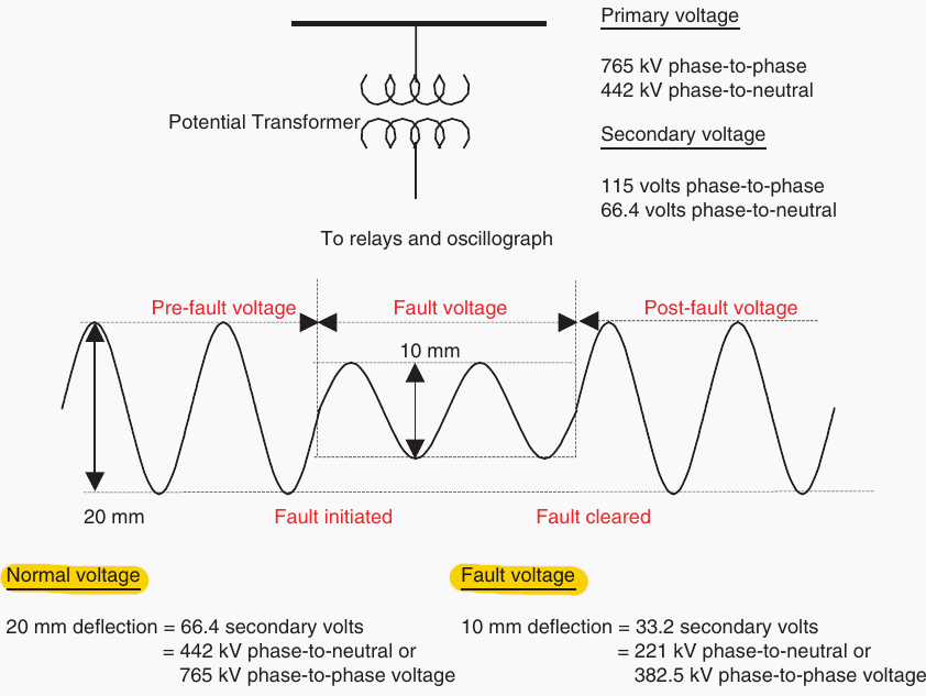
3. Voltage Reduction During Faults

Figure 1 depicts how an oscillogram can be used to determine the normal operating voltage and the voltage reduction during a fault. In this figure there are two cycles of prefault voltage, two-and-a-half cycles of reduced fault voltage and then voltage recovery to normal voltage after the fault is removed.

In the actual oscillogram, the trace would continue to the end of the record, which is normally set for 60 cycles.

Go back to Content Table ↑

4. Phase-to-ground Fault

Figure 2 depicts the traces associated with a phase-to-ground fault. There are one-and-a-half cycles of prefault normal load flow and two cycles of increased current during the fault. When the local breaker opens there is a redistribution of fault current. Although the total fault current will be reduced, the contribution from either end may increase due to infeed.

Figure 2 shows this increase from the local end until the remote end opens when the fault is cleared. Prior to the fault, there is no ground current. Actually, as discussed above, there may be some slight ground current trace due to unbalance.

The first breaker to open will remove the fault current from that end of the line while the remote oscillogram will continue to show fault current. The first breaker to close will result in an indication of charging current until the other end closes and load current is restored.

Since the phase current trace must accommodate the normal prefault load current while the ground current trace sees only the small prefault system unbalance, the two traces are calibrated differently.

Figure 2 – Phase-to-ground fault

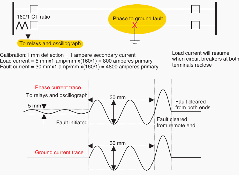
Figure 2 shows only two cycles of fault current which is the time it takes for the relays and the circuit breaker to operate and clear the fault. This is only an illustrative example.

Actually, in high voltage (HV) and extra high voltage (EHV) systems, with 3-cycle breakers and nominal 1-cycle relays, a fault should be cleared in about 5 cycles. Any longer time than this would alert the relay engineers to inspect either the relays or the circuit breaker. Of course, slower breakers or relays would take longer.

Figure 2 also shows how to calculate the secondary and primary load and fault current from the oscillogram. These values can then be compared with planning and short-circuit studies to verify the system values that have been used.

Go back to Content Table ↑

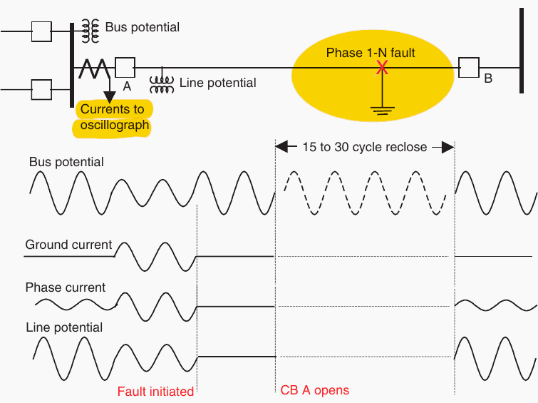
5. Phase-to-ground Fault and Successful High-speed Reclose

Figure 3 depicts a successful high-speed reclose (HSR) of circuit breaker (CB) A following a phase-to-ground fault on line A–B. Note that both bus and line potentials are recorded. This is very useful and common.

Since most faults are line faults, the bus potential would be a continuous trace, although the magnitude would be reduced during the fault. This provides a convenient timing trace. Referring to the figure, note that the line potential trace goes to zero when circuit breaker A opens but the bus potential trace continues and allows us to determine the HSR time.

In actual oscillograms, such as those in the literature,2 the information shown during the transition from prefault to fault, during the ‘dead time’ and after the reclose can be very significant.

Some of these interesting phenomena are shown in the figures below.

Figure 3 – Single phase-to-ground fault with successful high-speed reclosing (CB A, circuit breaker A)

Go back to Content Table ↑

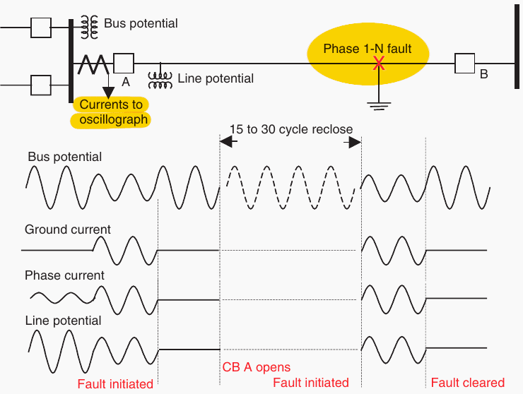
6. Phase-to-ground Fault and Unsuccessful High-speed Reclose

Figure 4 depicts the same situation as Figure 3 except that the fault is not temporary and reappears when the line is re-energized. The reclose is, therefore, unsuccessful and the line trips out again. The traces after the reclose are a repeat of the initial fault.

Figure 4 shows a typical switching transient in the bus potential trace.

Figure 4 – Single phase-to-ground fault with unsuccessful high-speed reclosing (CB A, circuit breaker A)

Go back to Content Table ↑

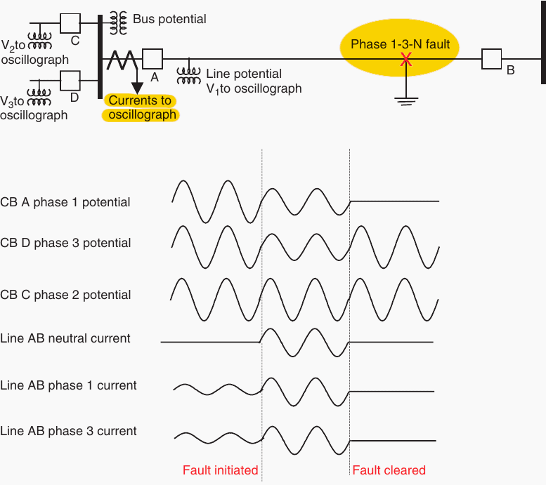
7. Analyzing Fault Types

For illustrative purposes we have shown only one phase current and voltage in the previous figures. Actually, we want to see, if possible, all three phase currents and voltages in a given line to determine which phases were faulted. This may require more traces than are available so some compromises are necessary.

Since the voltages during a fault will be the same throughout the station, a common practice is to record a different phase for each line. Also, by recording phases one and three and the ground current on each line all fault types can be determined.

Go back to Content Table ↑

7.1 Example

Referring to Figure 5, note that, when the fault occurs, the voltage traces of phases 1 and 3 are reduced, phase 2 is normal, phase 1 and 3 currents of line AB are increased and ground current appears.

These are clear indications of a phase-1-to-phase-3-to-ground fault on line AB. If there were no ground current we would conclude that it was a phase-1-to-phase-3 fault.

Figure 5 – Phase-to-phase-to-ground fault

Go back to Content Table ↑

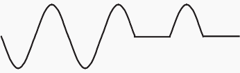
8. Circuit Breaker Restrike

Figure 6 shows how to determine that a breaker requires maintenance by the fact that it is restriking, i.e. the insulating medium is degraded or the contacts are out of adjustment so that current flow is reestablished even though the breaker contacts have separated.

Another indication, not shown in this figure, might be the presence of high-frequency signals as the contacts begin to close or open. Depending upon the frequency response of the fault recorder, we might see the actual waveshape or just a fuzzy record, but definitely not a clean 60 Hz trace.

This is an indication that an arc is being established or maintained through the insulating medium.

Figure 6 – Circuit breaker restrike

Go back to Content Table ↑

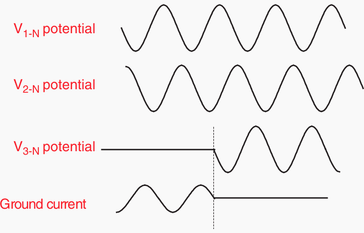
9. Unequal pole closing

Figure 7 shows an oscillogram of the three phase-to-neutral potentials and the ground current associated with closing a circuit breaker. There is always a certain amount of lag between the poles of a circuit breaker closing. This is normally of the order of milliseconds. It is a function of the breaker mechanism and is checked periodically by timing tests.

In Figure 7 the lag is equal to two cycles. As shown, ground current flows during this time and it is possible that ground relays will operate.

Figure 7 – Circuit breaker unequal pole closing

Further Study – Intricacies of a breaker pole discrepancy and its implications for substation operation

Intricacies of a breaker pole discrepancy and its implications for substation operation

Go back to Content Table ↑

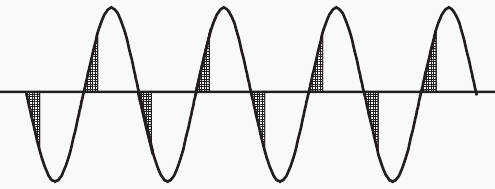
10. CT Saturation

Figure 8 shows the wave shape of a severely saturated CT. The shaded portion of the current wave is the current delivered to the relay.

The remaining portion is shunted to the magnetizing branch of the CT.

Figure 8 – CT saturation

Useful Tool – Current transformer (CT) saturation calculator

Current transformer (CT) saturation calculator

Go back to Content Table ↑

[be]

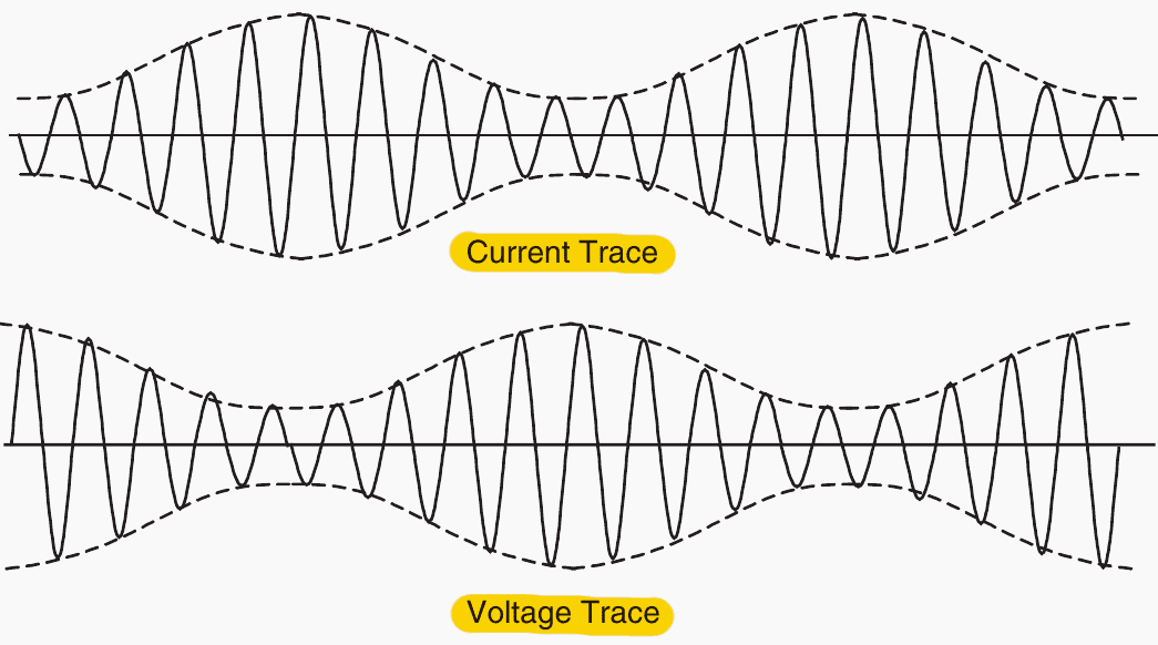
11. Power System Swing

Figure 9 shows the voltage or current during a system swing. The periodic oscillations in voltage and current magnitude indicate that various generators in the system are attempting to fall out of step with each other.

Figure 9 – Power system swing

Go back to Content Table ↑

12. Modern Digital Fault Recording Solution

The growing number of phasor measuring units (PMUs) in the electrical grid has led to a rise in the use of oscillation detection approaches based on phasors. The provision of voltage, current, frequency, and consequently power measurements at data rates that can readily hit 100 to 120 frames per second makes phasors an attractive choice for this application.

Given their role as the basis for detection algorithms, it is essential to comprehend and verify that phasor measurement techniques are appropriately suited for these situations.

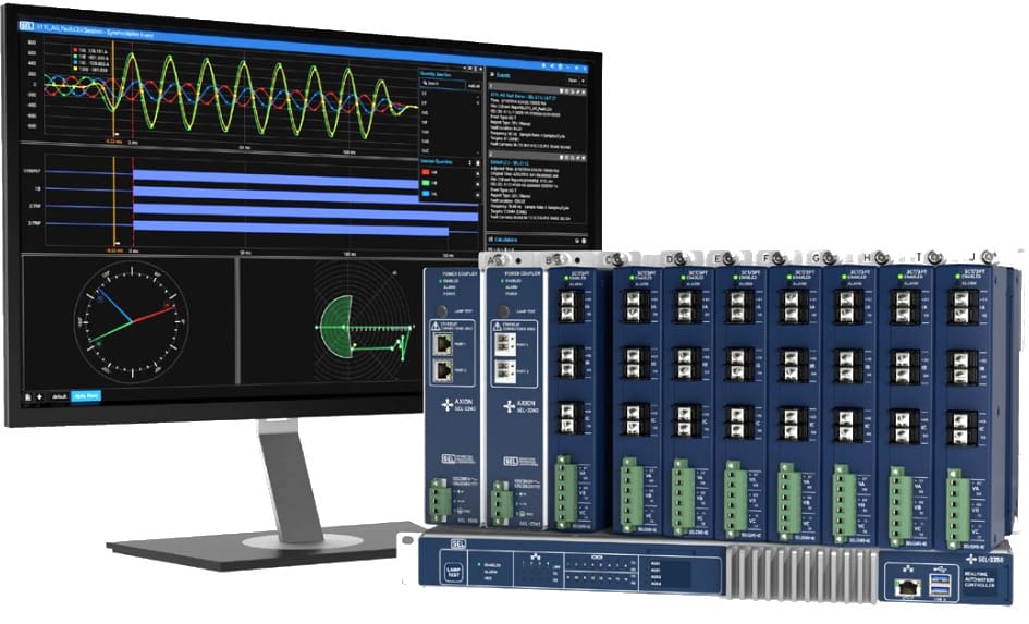
Figure 10 – SEL’s Advanced Digital Fault Recorder (DFR)

12.1 Applications of Digital Fault Recorder (DFR)

Record Disturbances and Exceed NERC PRC-002 Requirements

Collect power system data to facilitate event analysis and locate faults. Effortlessly exceed criteria such as NERC PRC-002. SEL’s  sophisticated DFR solutions generate and collect event reports, capture synchrophasors for dynamic disturbance data, capture SOE data, and determine fault locations with an impedance-based methodology.

Stream and Record Continuous Oscillography

Advanced DFR technologies provide continuous oscillography streaming and recording at 3 kHz, offering considerably enhanced insight into power system dynamics compared to intermittent event reports.

For example, SEL’s solutions utilize the Axion Wave Server for oscillography streaming and the robust RTAC logic engine for oscillography recording. The RTAC, equipped with 2 TB of local storage, facilitates uninterrupted oscillography recording at 3 kHz for a duration exceeding 10 consecutive days.

SEL’s sophisticated DFR systems provide extensive recording durations for various analog data, including synchrophasors from any phasor measurement unit (PMU) clients.

Figure 11 – Complete Solution With Supporting Software

Proactively Monitor Substation Assets

The RTAC logic engine not only executes essential DFR activities but also facilitates advanced monitoring of substation assets, including CTs, PTs, and networks. Custom logic can also be configured to facilitate applications such as monitoring circuit breaker wear.

Measure Energy With Greater Precision

Conventional phasor-based measurements depend on steady-state conditions. SEL’s industry-exclusive energy packet technology accurately measures energy flow under all system conditions, irrespective of frequency, angle, or distortion.

Utilize the RTAC logic engine to process Axion Wave Server samples for the calculation, streaming, and recording of energy packets.

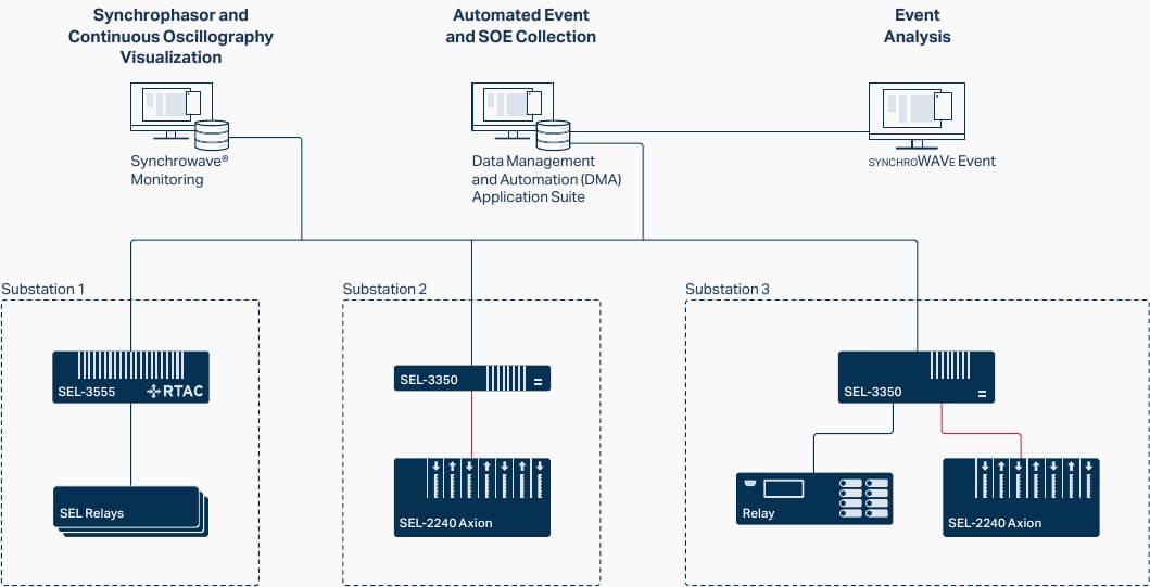
Figure 12 – Integrated DFR solutions

Refering to Figure 12, integrated DFR solutions use the RTAC to collect event reports and SOE data from IEDs and continuously record dynamic disturbance data streamed by IEDs. Leverage existing systems with SEL relays and other IEDs to perform dynamic disturbance and fault recording that exceeds standards such as NERC PRC-002.

12.2 Key Benefits of Digital Fault Recorder (DFR)

Disturbance Monitoring and Archiving for Compliance

Integrate historical synchrophasor data, continuous waveform streams, and event reports into a single display for a comprehensive disturbance monitoring system. Automatically identify system disturbances and export data in CSV and COMTRADE formats to facilitate compliance with NERC PRC-002-2, PRC-0028-1, and IEEE 2800 standards.

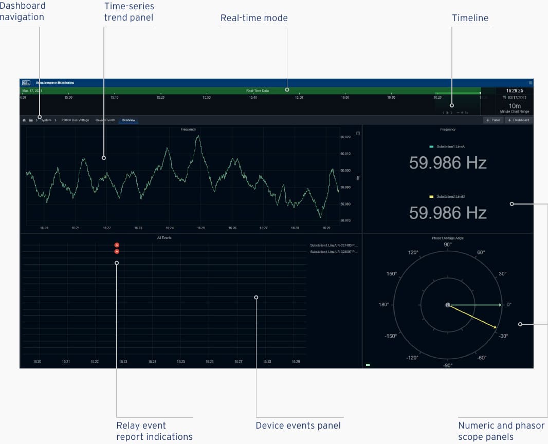
See the Real-Time System State

Improve system visibility by viewing live and time-aligned information from across the entire power system. Acquire further understanding of the power system’s dynamic behavior through waveform fingerprints to facilitate analysis under abnormal conditions.

Figure 13 – User Interface of Synchrowave Monitoring software

Validate and Improve Power System Models

To accurately replicate events, power system studies rely on accurate system models. Synchrowave Monitoring records the system response to system events, such as capacitor switching, generator trips, load shedding, or other events. Comparing the recording to system models enables engineers to plan a safer and more reliable system.

System dynamics from these generation sources change quickly—too fast to see at traditional SCADA rates.

Record and Analyze Continuous Waveforms

Never miss an event again. SEL provides a line of hardware that streams continuous waveforms in real time, including the SEL-2240 Axion, the SEL Real-Time Automation Controller (RTAC), the SEL-735 Power Quality and Revenue Meter, and the soon-to-release SEL-T35 Time-Domain Power Monitor.

Sampling and streaming rates range from 3 kilosamples per second (ksps) to 14.4 ksps. Synchrowave Monitoring software receives these data streams, provides real-time metering values, trends these values, provides real-time alarms, and archives the data.

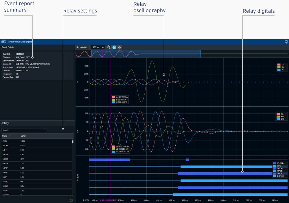
Figure 14 – Synchrowave Event Express: web client-based relay event report analysis software

Customize Calculations

View and customize a suite of power monitoring measurements. Virtual metering calculations utilize the 3.0–14.4 ksps data streams to provide power metering measurements, including voltage, current, power, frequency, symmetrical components, and power factor.

Additional power quality measurements include harmonics; RVC; voltage sag, swell, and interruption (VSSI); and flicker. The virtual metering application also calculates phasor measurement unit (PMU) quantities from continuous waveform streams.

Suggested Course – Power System Analysis, Modelling, Load Flow and Fault Studies for True Engineers

13. Summary

It is, of course, not practical to give examples of all of the information that oscillograms provide. However, some of the interesting system parameters that are recorded during system operations and should be studied whenever the opportunity presents itself are:

1. Unequal DC offset in fault current;
2. Trapped charge oscillations;
3. Line discharge through a CVT;
4. Ferroresonance;
5. Magnetizing inrush;
6. Evolving faults.

Reommended – Standard Operating Procedures (SOPs) for GIS Substations You MUST Fully Respect

Standard Operating Procedures (SOPs) for GIS Substations You MUST Fully Respect

Go back to Content Table ↑

13. Attachment (PDF): Power System Protection Handbook

Download: Power System Protection Handbook (for premium members only):

Go back to Content Table ↑

Sources:

1. Power Oscillation Detection and the Impact of Phasor Measurement Techniques by AMETEK
2. Power Quality Event Detection – Standards & Beyond by AMETEK
3. Advanced Digital Fault Recorder (DFR) Solutions by SEL