
Estimated Study Time: 28 minutes
Introduction to load shedding
Load shedding is a controllable reduction of a predetermined amount of the load power consumption according to specific shedding criteria. The predetermined amount of load to be shed is traditionally determined according to an analysis of the dynamic security for a set of contingencies. In this case, look-up tables are prepared and the implementation of the load shedding is performed according to them.
 The art of load shedding and online applications in a power system under an emergency state
A shedding lookup table is dependent on the operating conditions of the systems, its available topology, the available reserve, and the contingency. In addition, a look-up table must be updated for changes in the system. A look-up table determined for given operating conditions and a specific set of single contingencies might be not valid in the situation of multiple contingencies such as cascaded outages of lines.
The main objective of the load shedding is correcting an abnormal system state (explained in Section 2) to either the normal state or the alert state. For example, the balance of the generation and the load during abnormal operating conditions is a way for keeping the system’s stability.
- Reasons for load shedding
- Power System Security and the System States
- Under Voltage Load Shedding (UVLS) Schemes
- Under Frequency Load Shedding (UFLS) – An Overview
1. Reasons for Load Shedding
The load shedding can be applied manually or automatically. In addition, automatic load shedding has many philosophies. For example, the automatic reactive load shedding depends on the value of the absolute frequency as a shedding criterion while with the proactive load shedding not only the absolute frequency is used as a shedding criterion but also the rate of change of frequency or even the acceleration of frequency.
Based on its definition, load shedding is a corrective action by which system overloads can be relieved. The system overload can be classified according to its root causes as:
1.1 Active Power Shortage
In this case, the available power production sources or generators are insufficient to meet the system demand. In this case, the main symptom of system overload is a drop in the average system frequency. The shedding criterion, in this case, is the value of the system frequency. In the frequency drops below a predetermined value, the load shedding is activated.
This is called Under Frequency Load Shedding (UFLS).
1.2 Reactive Power Shortage
In this case, the available capacity is capable to meet the load active power demand while the voltage at specific locations in the network is too low for appropriate power flow and load requirements. The shedding criterion, in this case, is the violation of the bus voltage magnitudes.
For this purpose, it is called Under Voltage Load Shedding (UVLS).
Based on their time-frames and magnitudes of the associated changes in the operating conditions, system overloads may be also classified as:
1.3 Sudden and Large Changes
In this case, a disturbance causes the system to rapidly move from the initial stable operation conditions, and the time needed to take appropriate corrective actions before a possible system collapse is very small. In this case, fully automated, fast, and appropriate corrective actions must be taken.
1.4 Slow and Small Changes
In this case, a disturbance causes slow changes with small amplitudes. Consequently, manual corrective actions are possible. Based on this classification, the appropriate load shedding scheme can be determined.
The UVLS schemes are integrated into utility electrical systems to operate as a last resort for the controllable shedding of specific amounts of loads at specific locations in the grid. This action can prevent the loss of a large amount of the load or the entire load due to uncontrolled cascading events.
In contrast, the UFLS is designed for use in either emergency or extreme states (see section 2).
The goal of a UVLS scheme is to shed load to restore reactive power relative to demand, to prevent voltage collapse, and to contain a voltage problem within a local area rather than allowing it to spread in geography and magnitude. Load shedding is generally applied in steps. In each step, a specific amount of the load is dropped. If the first load-shedding step does not allow the system to rebalance, and voltage continues to deteriorate, then the next block of the load is dropped.
The UFLS operates in the same manner.
2. Power System Security and the System States
Power system security may be defined as the continuous ability of the power system to keep all the system limits not violated with minimum interruption to the supplied loads. The main target of the power system security is to keep the system intact under normal and disturbed conditions. Therefore, a successful security system should minimize the impact of disturbances on the operation, economics, and power quality of power systems.
In addition, an acceptable system security level guarantees the immunity of the power system to disturbances and makes the system defensive. Therefore, secure operation of power systems requires the integration of all practices designed for keeping acceptable system operation when components fail.
Power system security covers both static and dynamic phenomena. Therefore, the security analysis is usually categorized into static (or adequacy) and dynamic security. Static security considers the impact of static or slow changes in the system limits while dynamic security considers the impact of disturbances (or contingencies) on the system.
The core definition of dynamic security and stability is the same, but the security is a wider term than stability.
System Stability Definition
Stability is defined as:
“The ability of an electric power system, for a given initial operating condition, to regain a state of operating equilibrium after being subjected to a physical disturbance, with most system variables bounded so that practically the entire system remains intact”; however, “Security not only includes stability but also encompasses the integrity of a power system and assessment of the equilibrium state from the point of view of overloads, under- or over- voltages and underfrequency”.
The system limits define the normal operation of power systems. These limits or constraints can be classified into two categories; equality and inequality constraints. In addition, the system limits may be classified according to their origin into intrinsic limits and operating range limits. The equality constraints basically represent the load flow equations while the inequality constraints represent the allowable range of acceptable operation of various components in the system.
In fact, the intrinsic and operating range limits elaborates on the inequality constraints associated with a specific component. The intrinsic limits of equipment are determined basically from the design and characteristics of the equipment. The operating range limits are generally less than the intrinsic limits and they are limited by the fulfillment of the overall operational requirements of the system.
For example, consider a simple hypothetical system where an off-grid generating plant supplies a load center via a short transmission line with negligible impedance. The generator is capable of producing a voltage magnitude at its terminal in the range 85% – 115% while the load requires a voltage magnitude in the range 95% – 105%.
In this case, the generator voltage limits present the intrinsic limits of the generator and they are mostly related to its design. Successful operation requires that the voltage magnitude at the load bus should not be violated.
Therefore, the operating range limits of the generator bus-voltage magnitude becomes equal to the load requirements (i.e. 95% – 105%). It is worthy to be mentioned that the 95% – 105% voltage limits present an intrinsic limit as viewed from the load perspective.
It is also important to know that the operating range limits should not violate the intrinsic limits of any component within a system. Otherwise, the system will be incapable of fulfilling the operational requirements. Both intrinsic and operating range limits are not absolute constants. The intrinsic capability limits usually decline with time due to the degradation of the equipment.
For example, the annual output degradation rate of PV systems is about 0.7%. The degradation may be attributed to aging, operational stresses, and maintenance quality.
The operating range limits are also variable. For example, the ampacity (or ampere capacity or current limits) of a cable is highly dependent on the temperature of its surroundings. The ampacity limits are usually increased during the winter and decreased during the summer. This is for avoiding the over-temperature of the cable insulation.
Recalling that in the normal operation of a power system, all the inequality and equality constraints of the system are satisfied. In addition, the system security requires a minimum available, reserve margin. Power system security may also be defined as the ability of the system to withstand credible contingencies without violating the normal operating limits.
A system operating under normal conditions is also said to operate in the normal state. The security strength of the system is usually defined by the maximum number of time-independent, and simultaneous disconnection of major system components (such as generators, transformers, and lines) without affecting the normal operation of the system.
Defining N as the minimum number of components required to supply the system peak load. A system with an N-k security criterion is a system in which k components may be simultaneously disconnected and the system will be able to fulfill the normal state requirements in the post-contingencies time. Due to investment constraints, power systems are usually designed according to the N-1 security criterion.
The normal state is a secure state and a system operating in the normal state is said to be intact.
Deviations from the normal state requirements cause the system operation to move to insecure operating states. These deviations are mainly caused by contingencies which are stochastic and unexpected events; however, the rate of contingencies may be reduced for example by proper maintenance of components. Four insecure operating states can be realized.
These states are the alert, emergency, extreme (or collapse), and restoration states.

Figure 1 illustrates the main operational characteristics of these states and the interrelations between them. This figure is usually called the state transition diagram. Table 1 summarizes the characteristics of various states, some causes of state transitions, and examples of the corrective actions for each state. The nomenclature used in the table is illustrated in Figure 1.
It is worthy to be mentioned here that an intact system is capable of providing power balance. If the power balance could not be achieved, then the system becomes not intact. Consequently, the synchronization of generators upsets. Therefore, the system frequency protection devices will split the system into parts or islands; the situation is called islanding and it is within the extreme state.
Generally, delayed or unsuccessful corrective actions during the operation in any state may lead to severe consequences. Therefore, any security program includes a contingency analysis block. The contingency analysis is an investigative simulation of hypothesized contingency for evaluating their impact on system security.
On the other hand, the corrective action analysis is the process of figuring the possible actions that may be taken for overcoming the consequences of security upsetting contingencies.
Table 1 – Summary of operating states and state transitions
| State | E | I | N-1 | N | Intact System | Causes of transition from normal state | Corrective Actions |
| Normal | ✔ | ✔ | ✔ | ✔ | Yes | — | — |
| Alert | ✔ | ✔ | ✖ | ✔ | Yes | Constraints are near their limits. Examples, reduction in the reserve margin or bus voltage close to the limits. | Preventive control. Examples, startup of the nonspinning reserve or switching on compensators respectively. |
| Emergency | ✔ | ✖ | ✖ | ✖ | Yes | Severe disturbances. For example: short-circuit faults or cascaded outages. | Emergency control actions (heroic measures). Example: fast fault isolation or operation of reclosers. |
| Extreme | ✖ | ✖ | ✖ | ✖ | No | Delayed or unsuccessful emergency control actions. Severe power imbalance. | Heroic and remedial actions such as load shedding, generator trip, or intentional islanding for keeping power balance. |
| Restoration | ✖ | ✔ | ✖ | ✖ | No | The attempt of restoring the system to the normal state or at least to the alert state. | Manual or automated reinsertion of generators and loads. The inequality constraints should be kept satisfied during the entire restoration process. |
The corrective action analysis works in two distinct modes. The first mode operates for solving the problems found by the contingency analysis. Therefore, this mode is offline while the second mode operates in real-time operation for securing the system during its real-time operation.
The contingency analysis and the corrective action analysis require the simulation of the system. Therefore, an accurate system model should be available. In addition, the results obtained from these analyses are highly dependent on the accuracy of the system model. Real-time models of a power system require centralized real-time data collection available from local measuring and monitoring devices at each system component.
Therefore, telemetry is required for communication within the system and for estimating its state.
Recommended Reading – 5 telecommunication systems embedded in smart grid applications and services
Five telecommunication systems embedded in smart grid applications and services
3. Under Voltage Load Shedding (UVLS) Schemes
As a result of a disturbance, the voltage magnitude may drop to a preselected level for a predetermined time. In such cases, the UVLS sheds a selected amount of loads at selected locations in the system. The objective is then to prevent widespread voltage problems or voltage collapse. System planning engineers perform numerous studies (see Figure 2) using the PV curves as well as other analytical methods for the proper determination of the minimum amount of load that must be shed for securing the system to retain voltage stability under credible contingencies.
Various voltage control equipment provides a defense against voltage collapse; however, in situations, the system is subjected to severe disturbances or cascaded outages, various voltage control and voltage restoration equipment may fail to restore the normal state voltage range.
In these situations, the load shedding provides an effective corrective action for preventing either the voltage collapse or the islanding of the system.
This is illustrated in Figure 3. The shown voltage problems are attributed to the insufficiency of the reactive power sources needed for restoring an acceptable voltage level.

It should be noted that system operators usually shed load as the last resort.
Under Voltage Load Shedding (UVLS) schemes, drops a load when the voltage gets too low. The dropping of the load will alleviate the system by eliminating the current flowing to the dropped load. UVLS usually triggers distribution feeders to open when the voltage of the bulk electric system is around 90%. Definite time relays usually act when all three phases show low voltage for around 10 seconds at 90% voltage magnitude, this would be after some of the ULTC transformers have been acted.
Certain critical customers cannot be dropped from load despite the help it may present to the system. Critical customers include hospitals or customers that would lose lots of revenue from being dropped.
The order of various corrective events following a contingency is shown in Figure 3.

The events started as a response to a contingency such as a forced outage of a generator or a line. Erroneous operation or vandalism may also cause disturbances of a similar impact.
There are two main UVLS schemes:
- Decentralized (also called distributed UVLS) and
- Centralized schemes.
Figure 4 illustrates a typical distribution substation with integrated UVLS and UFLS special protections.
In this system, the UV relay is installed on the HV side of the transformer for the correct detection of the grid voltage. This is because the voltage on the secondary side is not a real indication of the grid voltage due to the actions of the ULTC transformer (or any other load side voltage controllers). The UF relay is installed on the LV side of the transformer because the transformer does not affect the frequency while the LVPT is more economical in comparison with the HVPT.
The main complication associated with the setting UVLS is the inaccuracies associated with the PT and the UV relay. Therefore, a proper and secure setting should be chosen for considering the probable inaccuracies.
4. Under Frequency Load Shedding (UFLS) – An Overview
In this section, an overview of the UFLS schemes and technologies will be presented. Generally, the system frequency is a good indicator of the power balance and overload
conditions in a power system. The UFLS is the last resort for the treatment of serious frequency declines in power systems when subjected to large disturbances.
Under the emergency state or the extreme state, the ability to maintain the power balance and stabilize the frequency is directly related to the effectiveness of the employed UFLS Strategy.
An effective UFLS strategy should be capable of:
- Restrain the frequency decline,
- Restore the normal frequency,
- Minimize the load shedding,
- Minimize the frequency recovery time,
- Minimize the frequency fluctuations, and
- Provide the desired protection functions as economical as possible.
Typically, a UFLS scheme sheds the loads in several stages. In each stage, a predefined amount of the load is disconnected and the shedding of the load is continued till the normal frequency (i.e. the power balance) is restored. This is illustrated in Figure 5 below.
The proper timing of shedding each load block should not only depend on the frequency but also the rate of change of the frequency. This results in an adequate time separation between the shedding of blocks.
Using small load shedding blocks in conjunction with shedding timing based on the rate of change of frequency can be an effective way to the prevention of over-shedding.

The blocks of load shedding shown in Figure 5 can be selected based on two criteria; the static criterion and the dynamic criterion. Figure 6 shows flowcharts describing the logic of each criterion. In the static criterion, fixed load blocks are disconnected in each load shedding stage. This criterion may reduce the impact and the effectiveness of the load shedding, especially in large disturbance conditions that are associated with a steep decline in the frequency.
The dynamic load shedding is constructed for solving this problem. In the dynamic load shedding the amount of load to be disconnected at each shedding stage is dynamically selected based on the system frequency, the rate of change in the frequency, the voltage, and the severity of the disturbance(s).
In other words, the amount of a load shedding block is a function of the magnitude of the power imbalance.

There are three main methods for the implementation of UFLS strategies. These methods are:
4.1 The traditional method
When the frequency is lower than the first setting value, the first level of load shedding will be implemented. If the frequency continues to decline, it is clear that the first load shed amount is insufficient. When the frequency is lower than the second setting value, the second stage of load shedding is then implemented. If the frequency continues to decline, the further load shed stages are activated until the normal frequency value is restored.
4.2 The semi-adaptive method
To some extent, this method is similar to the traditional method; however, the specific amount of load to be shed is determined in terms of the measuring value of the rate of change of frequency.
4.3 The self-adaptive method
The self-adaptive method follows the dynamic shedding criterion for a more accurate estimation of the proper amounts of the load to be shed in each stage and the timing of each stage.
Related electrical guides & articles


Mohamed EL-Shimy
Prof. Dr. Mohamed EL-Shimy is currently a professor of electrical power systems with the department of Electrical Power and Machines – Faculty of Engineering - Ain Shams University. He is also an electromechanical specialist, a freelance trainer, technical advisor, and a member of many associations and professional networks. He is a technical reviewer with some major journals and conferences. His fields of interest include electric power system: analysis, stability, economics, optimization, distribution, renewable energy integration, and reliability.Profile: Mohamed EL-Shimy

This a nice read and very interesting.Very insightful and concise.
Thanks prof.for the time to share your knowledge.
Collins.
very nice article,
thank you for your sharing …..
can you please clear it, in my plant load shedding on grid is prefixed, when grid trip load shed acts, its which type of load shedding.
thanks®ards,
venkatesh.
Appreciation with thanks, Prof. Mohamed El-Shimy for the valuable information.
Thank you for your encouraging feedback.
Am so happy to read about your professionalism it encourage me to study more even now that am still working in injection power station as an operator
Thanks Prof. Omar for sharing this wonderful information.
Thanks Prof. Mohamed for intersting article,
Best wishes,
Omar
Thank you Prof. Omar for your feedback.