
Estimated Study Time: 38 minutes
Modern Electrical Analysis
This technical article we will go through a number of existing applications for conducting a wide range of electrical studies. However, the practice says that studies involving load flow and fault analyses are the most commonly utilized programs in power transmission & distribution design and analysis.
 Ten most important calculations of power system analysis software
The software used for analyzing power systems might be as simple as a commercially available, generic package or as complicated as a custom-built application. The latter can be integrated in real time to an electrical SCADA system with real input from the field, and it satisfies the needs of a single comprehensive electrical system.
A load flow analysis analyzes the voltage, current, power, and reactive power at a variety of points and branches during simulated normal operation. Planning for future networks or additions to existing ones, as well as optimizing existing networks, all require load flow studies to provide an economically and efficiently distributed load.
Immediately following an electrical fault, the currents flowing into various portions of a power system deviate significantly from the currents flowing under steady-state conditions. The ratings of the circuit breakers and other switchgear in the system are based on the fault current and the current that the circuit breaker must interrupt immediately after the fault is cleared.
Predicting these currents for different fault types in different places is what fault computations are all about. Settings for protection relays are determined in part by data obtained from fault computations.
Power system automation systems provide real-time data that can greatly complement and supplement network analysis. First, the findings of load flow studies can benefit greatly from the steady-state information that is continually gathered, preserved, and trended.
Secondly, the data gathered from disturbance records and sequence-of-events recordings can be utilized to check the accuracy of fault calculations and stability studies, as well as the efficacy of electrical protection.
- Load Flow Study
- Conductor Sizing Study
- Transformer Sizing
- Fault Analysis
- Transient Stability Study
- Fast Transients Study
- Power System Reliability
- Relay Protection Schemes Analysis
- Arc Flash Study
- Power Quality Analysis
- Earthing Study
- To Conclude
- BONUS! Fault Current Calculator (XLSX) + Power Protection Analysis (PDF)
1. Load Flow Study
The load flow (or power flow) program was one of the first to be developed for power system analysis. It was first created in the late 1950s. Load flow programs are included in all full packages in use today because they are one of the foundations of any electrical network study.
Although an electrical network is linear, load flow analysis is iterative due to the interaction of voltages, currents, frequency, and reactance. The generators are programmed to provide a specified amount of active power to the system, and the voltage magnitude at the generator terminals is normally fixed via automatic voltage regulation.
In certain programs, this busbar is referred to as the slack bus or utility bus. The slack bus is a mathematical necessity for the software and has no real-world analogue.
In actuality, the total load plus losses are unknown and fluctuate on a constant basis. When a system is out of power balance, that is, when the input power does not match the load power + losses, the rotational energy stored in the system is altered. Thus, if the input power is too high, the system frequency rises, and if the input power is too low, the system frequency decreases.
Figure 1 – Load flow analysis of 138/69 kV substation using ETAP

Typically, a generating station with a single machine is tasked with maintaining a steady frequency by adjusting the input power. The first algorithms offered the advantages of simple programming and minimal storage, but they were slow to converge and required many iterations. The introduction of ordered elimination of the network matrix, as well as programming techniques that reduced storage needs, enabled the adoption of considerably superior algorithms.
The Newton-Raphson approach provided solution convergence in a few iterations. A Jacobian matrix containing the partial derivatives of the system at each node can be generated using Newtonian methods of problem specification.
The rapid decoupling technique requires more iterations to converge but consumes less computational effort per iteration than the Newton-Raphson method.
A load flow study’s results can be viewed as a snapshot of the system once steady-state conditions have been reached with all loads being constant. The research computes the voltage on each bus, the voltage drop on each feeder, the current, power flow, and losses in each branch, and the total system losses. Load diversity concerns can be included in branch loads.
Suggested Course – Power System Analysis, Modelling, Load Flow & Fault Studies
Power System Analysis, Modelling, Load Flow and Fault Studies for True Engineers
2. Conductor Sizing Study
The sizing analysis chooses the conductor size based on the minimum conductor material and cross-sectional area required to achieve the stipulated feeder current-carrying capabilities and associated voltage drop standards. This helps ensure that the conductor will not experience any voltage drop.
The kVA rating of a transformer at full load is used to determine its size.
2.1 Feeder Sizing
Feeder sizes are determined by the demand load study’s design load value. The demand load analysis computes the total connected demand and design load in each power system branch. Because some loads are designated as continuous loads, their design load value is greater than their demand load value.
Branch circuits that service continuous loads must be rated so that no more than 80% of the feeder current rating is used, according to the NEC. The NEC standard is met by selecting a design load value of 125% of the demand load value. The feeder current rating is defined as the maximum continuous current in amperes that a conductor may carry without exceeding its temperature rating.
To be available for the sizing research, cable sizes are typically listed in a cable library.
The temperature derating factor and the duct bank design detail criterion are used to calculate derating factors.
The sizing study determines the cable with the smallest cross-sectional area that best matches the defined current rating values. After selecting the cable, the voltage drop for the cable or cable pair is determined. If the voltage drop threshold is surpassed, the sizing study moves on to the next bigger cable size and compares cross-sectional area, rated current, and voltage drop.
Figure 2 – ETAP cable sizing software
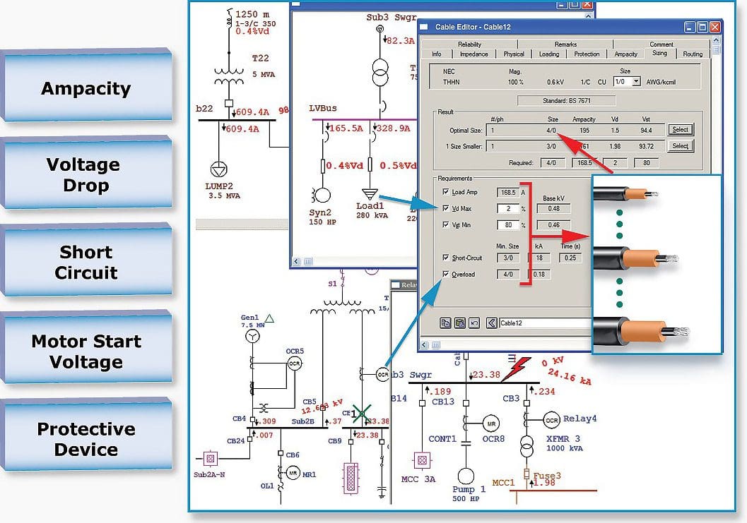
The feeder branch design load value in amperes is determined by the sizing study methodology, which then determines the appropriate feeder design current rating. The product of the rated current, the temperature derating factor, and the number of parallel wires yields the feeder design rating.
The design load value is calculated by multiplying the rated size of the load by the prescribed demand factors and the long continuous load factor (or design factor).
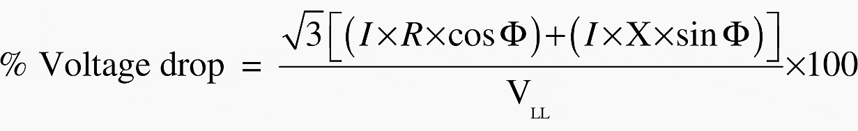
Once the current rating parameters have been met, the sizing study examines the calculated voltage drop on the cable, which is based on the branch design load current and power factor, cable impedance, and length.
The voltage drop can be calculated using the following formula:
If the voltage drop is found to be unacceptable, the sizing study will choose the next largest feeder and then begin the process again in order to choose a cable or combination of parallel cables that satisfies the rating criteria of having a minimum cross-sectional area and an acceptable voltage drop.
Suggested Guide – Placement and rating planning of feeders & transformers for LV/MV distribution networks
Placement and rating planning of feeders & transformers for LV/MV distribution networks
3. Transformer Sizing
Depending on the user’s preference, the size of the transformer is often determined by either the calculated demand of the branch or the design load value. The demand load value or the design load value is compared to the full load size of the transformer by the sizing algorithm.
The transformer’s full load size is:
Full load size = Nominal kVA rating × Transformer capacity factor
Table 1 – Typical capacity factors for transformer cooling characteristics
| Transformer Cooling Characteristic | Capacity Factor |
| Dry type (DT) | 1.00 |
| Oil/air cooled (OA) | 1.15 |
| Oil/air/forced air (OAFA) | 1.25 |
3.1 Transformer Feeders
The primary and secondary feeders of transformers are designed with a factor (often 125% of the transformer’s full load rating) and a tolerable voltage drop criterion in mind. This factor is often defined in the dialogue box that is used to set up the demand load research.
4. Fault Analysis
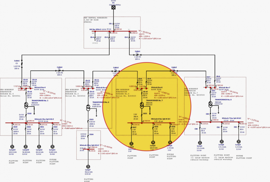
The development of a fault analysis program arises from the necessity to accurately assess the capacity of switchgear and other busbar equipment to withstand the highest available fault current that may pass through them.
By including the outcomes of a load flow analysis prior to conducting the fault analysis, it becomes possible to incorporate the load currents alongside the fault currents, hence enhancing the precision in determining the overall currents present within the system.
Figure 3 – Device Duty Calculations using ETAP’s short circuit analysis software
The inclusion of unbalanced faults can be achieved through the utilization of symmetrical components, which involves the mathematical division of fault currents into negative sequence, positive sequence, and zero sequence currents.
In the process of calculating fault levels in an industrial plant, it is imperative to include the contributions of motors and generators! The impact of their contribution to the fault current can have a substantial effect on the ultimate value. Contemporary software applications also consider the Direct Current (DC) effect.
Figure 4 – Short circuit analysis using ETAP software (click to zoom)
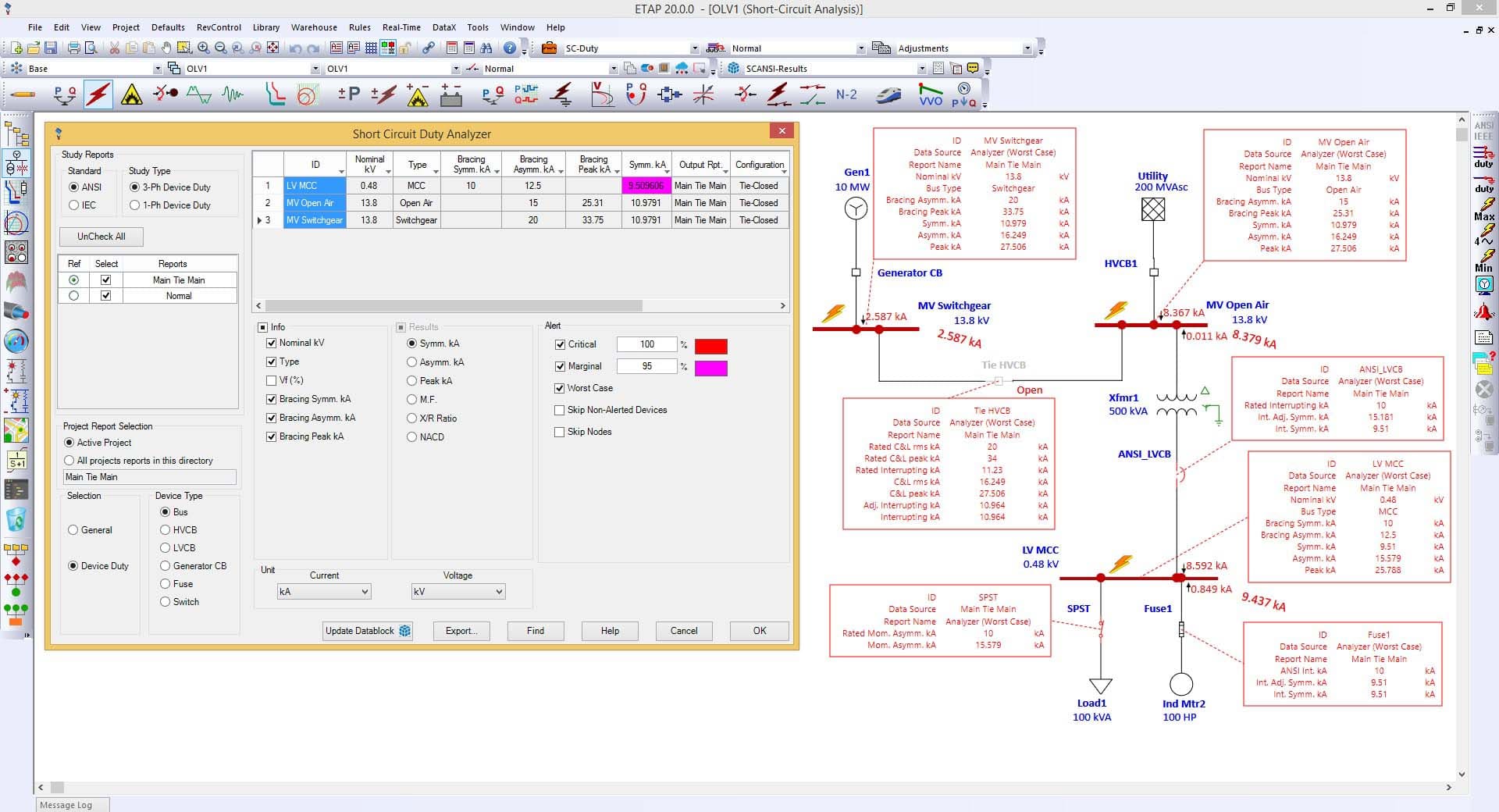
Through the use of Short Circuit Analysis, you will be able to assess the effect of balanced and unbalanced faults, as well as automatically compare these values to the short circuit current ratings provided by the manufacturer.
Utilizing analyzers, graphs, and reports, you can swiftly ascertain both the optimal and the worst-case fault current device duty.
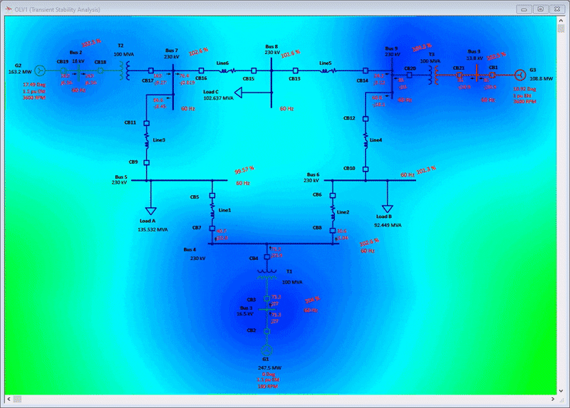
5. Transient Stability Study
Following a disturbance, typically caused by a network fault, the electrical loading of the synchronous machine undergoes changes, resulting in an increase in its speed (although in very modest loading conditions, it may experience a decrease in speed). The response of each machine will vary based on factors such as its distance from the fault, its initial load, and its time constants.
This implies that the angular orientations of the rotors with respect to one another undergo alterations. When an angle beyond a specific threshold, often ranging from 100° to 140°, the machine’s ability to sustain synchronism becomes compromised. The consequence of this action typically entails the removal of the service.
The initial research efforts in the field of transient stability mostly focused on investigating the response of a single synchronous machine that is interconnected with a significantly large power supply via a transmission line.
The assumption can be made that the huge system is of unlimited size in comparison to the single machine, allowing it to be represented as a pure voltage source in the model.
Figure 5 – Transient stability analysis enables engineers to accurately simulate and analyze power system dynamics and transients via system disturbances and other events
The synchronous machine can be represented by the stator’s three-phase windings, along with windings on the rotor that symbolize the field winding and the eddy current channels. The resolved components can be classified into two axes: one aligned with the direct axis of the rotor, and the other aligned with the quadrature axis, which is positioned at a 90° (electrical) angle from the direct axis. The field winding is located along the direct axis.
Equations can be derived to ascertain the voltage in a given winding based on the current flowing through all other windings. It is possible to generate a comprehensive system of differential equations that enables the determination of the machine’s reaction to varied electrical disturbances.
The factors that need to be included are rotor angle and rotor speed. One notable drawback associated with this particular analysis is the perpetual variation in rotor location due to its continuous rotation. Due to the presence of trigonometric functions pertaining to stator and rotor windings in the majority of equations, it is imperative to consistently reassess the matrices.
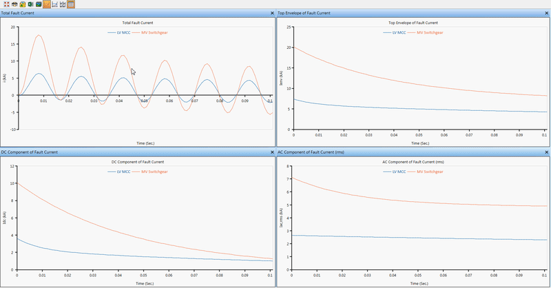
Figure 6 – Transient stability graphs
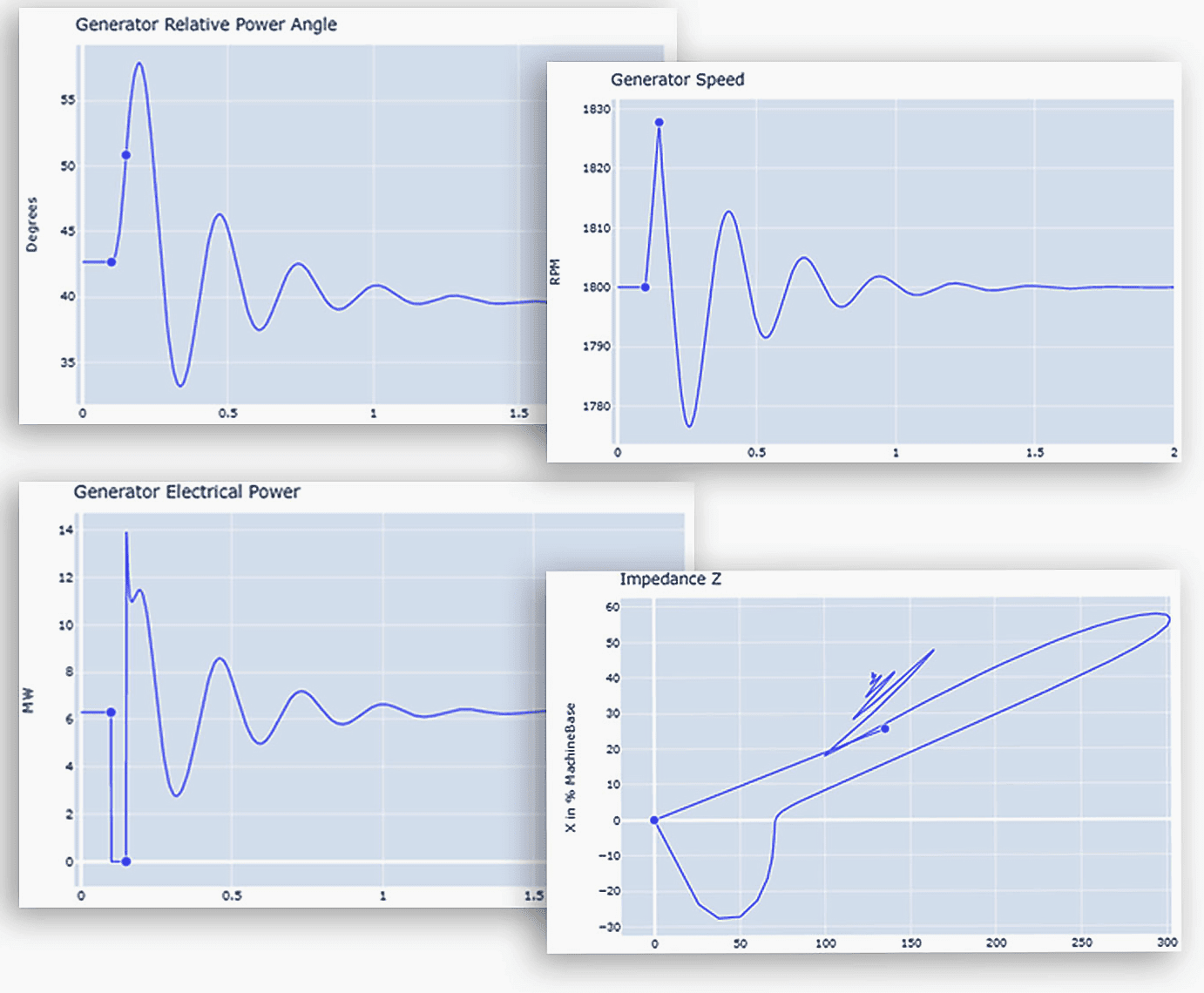
In instances where network faults are particularly severe, the outcomes become balanced once the direct current transients have dissipated. Moreover, once the defect is eliminated, the network is seen as being in a state of balance. The acquisition of comprehensive data for each of the three stages requires a significant amount of computational effort, which holds little significance for power system engineers.
In contrast, the significance of this form of study is paramount for machine designers. Nevertheless, this technology has been utilized to develop programs for multi-machine systems.
Contemporary programs also include the system’s response, not alone in response to significant disruptions, but also in relation to the accumulation of oscillations caused by minor disturbances (such as asynchronous resonance) and inadequately configured control systems.
When determining the system’s response to disturbances, it is not appropriate to rely solely on lengthy time domain solutions. Therefore, frequency domain models were constructed to address this issue.
Suggested Course – Power System Modeling and Stability Analysis Using ETAP
Power System Modeling and Stability Analysis Using ETAP – Beginner to Advance Level Course
6. Fast Transients Study
The transient stability program takes into account the dynamic behavior of the power system throughout the frequency range of 1 to 10 Hz. However, it is also necessary to compute the system’s reaction to rapid changes in conditions, such as transitioning between different switching ranges, as well as the propagation of intense voltage and current waves through transmission lines caused by a lightning strike.
In order to accurately represent these effects, it is imperative to employ a highly comprehensive model that encompasses all stray capacitances and inductances. A significant proportion of these programs exhibit a high level of complexity in terms of usability and need a substantial amount of time to resolve.
Due to this rationale, it is customary to primarily investigate brief time intervals.
Recommended guide (PDF) – Transient behavior of substation grounding grids under lightning surges
Transient behavior of substation grounding grids under lightning surges
7. Power System Reliability
The operators of power systems are consistently concerned about the reliability of equipment. Historically, the assurance of dependability was achieved through the implementation of backup equipment, either operating in parallel with comparable devices or capable of being swiftly linked in the case of a malfunction.
Nevertheless, the provision of additional equipment to accommodate unforeseen circumstances has become increasingly expensive as systems continue to grow.
The assessment of reliability indicators at the generation and transmission levels primarily includes the loss of load expectation and the evaluation of frequency and duration. The conventional way to assessing reliability indicators at the distribution level, such as the average interruption ratio per customer per year, often involves employing an analytical methodology centered around a failure-mode evaluation.
Recommended Paper (PDF) – Reliability of the electric power distribution system for six alternative loop configurations
Reliability of the electric power distribution system for six alternative loop configurations
8. Relay Protection Schemes Analysis
The necessity to examine protection schemes has led to the emergence of protection coordinating programs. Protection schemes can be categorized into two primary classifications: unit schemes and non-unit schemes.
The initial category encompasses protective methods designed to safeguard individual components within the system, such as transformers, transmission lines, generators, or busbars. One prominent illustration of unit protection strategies is founded on Kirchhoff’s current law, which states that the total sum of currents flowing into a certain region of the system must equate to zero. Any departure from this standard would suggest an atypical flow of electrical current!
Within these frameworks, the consequences of any perturbation or operational circumstance beyond the designated scope are entirely disregarded, necessitating the creation of protection mechanisms that maintain stability even when subjected to the highest conceivable fault current that may traverse the safeguarded region.
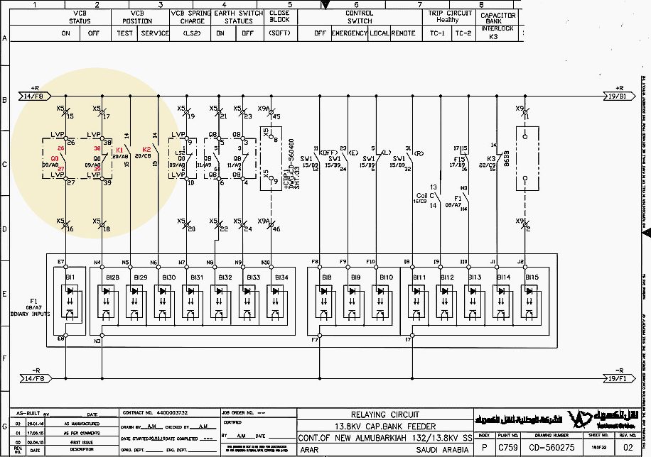
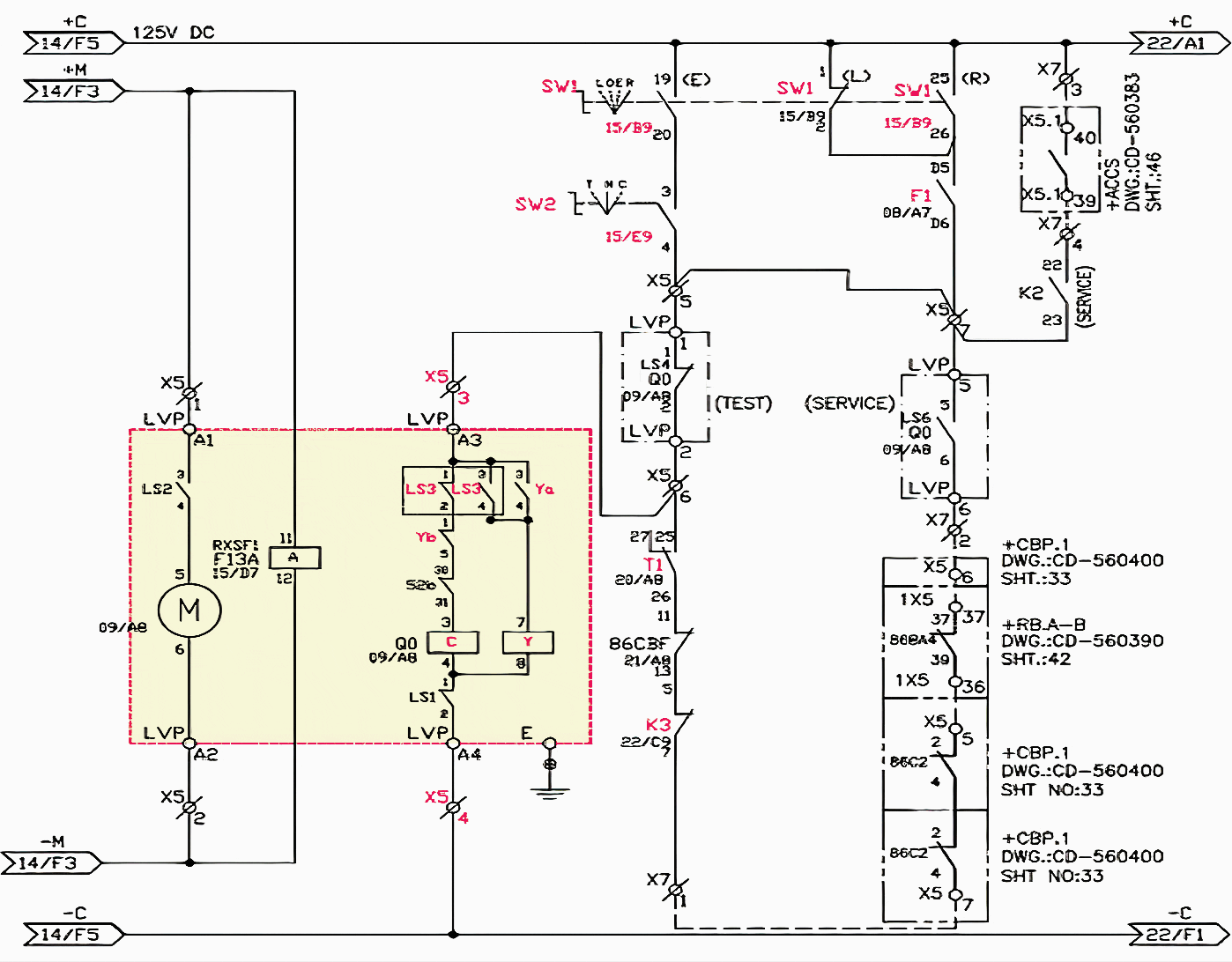
Figure 7 – BCPU and Alarm Signals (click to zoom schematics)
Schemes may be devised to encompass all facets of a transformer in order to accommodate the varying currents at distinct voltage levels. Therefore, the examination of these systems holds greater significance for makers of protective equipment.
The non-unit plans, although designed to safeguard particular regions, lack defined demarcations. In addition to safeguarding their respective designated regions, the protective zones have the potential to extend into overlapping territories. Although the utilization of backup systems might offer significant advantages, it is important to acknowledge the potential drawback of excessive isolation in the event of a fault being identified through various non-unit schemes.
One of the simplest methods among them measures the current and includes an inverse time characteristic into the protection process, enabling the protection closer to the fault to activate first. Setting protection in networks can be challenging due to the varying current routes caused by varied operating and maintenance procedures.
While it is relatively simple for radial schemes, achieving optimal settings is likely unattainable.
Figure 8 – Circuit breaker closing circuit (click to zoom the schematics)
Protection software has proven to be beneficial for manufacturers, consultants, and utilities in several specific domains.
The nature of protective systems has seen a significant transformation, progressing from electromechanical devices to electronic counterparts that mimic the functionality of their predecessors, and ultimately evolving into advanced system analyzers known as microprocessor-based relays or intelligent electronic devices (IEDs).
Computers possess inherent autonomy, rendering them capable of being predominantly advanced through the utilization of computer analytic methodologies.
Recommended Course – Learn AC Distribution Panel Drawings: Single-Line Diagrams, Wirings, and Interlocking Schematics
Learn AC Distribution Panel Drawings: Single-Line Diagrams, Wirings, and Interlocking Schematics
9. Arc Flash Study
High-risk arc flash locations in an electrical system can be located and analyzed with the help of Arc Flash Analysis software, which also allows for the modeling of a variety of techniques used by engineers to reduce the effects of arc flashes. With this comprehensive software, you may set out a number of different situations to find the one that results in the most incident energy.
It also offers a number of options for producing reports and arc flash labels of publication grade.
You may quickly and easily find out which possible outcomes are the worst with the use of such time-saving technologies. Warnings and problem regions can be filtered out with the help of the arc flash analyzers.
Good Reading – Do you know what an arc flash is? If not, keep reading, it’s important.
Do you know what an arc flash is? If not, keep reading, it’s important.
Some arc flash applications, in addition to 3-phase systems, allow you to perform arc flash calculations for 1-phase systems. This tool allows you to estimate the incident energy for single phase arc faults conservatively. The reality is that much of the equipment is single phase, and engineers must still establish what energy levels are possible at these sites.
The engineer can use this technique to produce a conservative estimate of that energy.
Some of the features of Arc Flash programs:
- Sort results from different studies by multiple criteria.
- Find the worst-case incident energy results.
- Quickly identify incorrect sequence of protective device operation.
- Determine which protective devices failed to operate.
- Filter and analyze results by incident energy levels.
- Recognize slow operation of protective devices.
- Run several arc flash simulations with a single click and examine the results in seconds.
- Define your own parameters or use system-calculated results to assess incident energy.
Useful Calculator – Electrical Safety Program Arc Flash Calculator
10. Power Quality Analysis
There are many harmonic analysis programs available currently, and high harmonic levels are sometimes regarded as a symptom of poor power quality. Over the last two decades, the use of non-linear loads such as arc furnaces, HV DC converters, FACTS equipment, DC motor drives, and variable AC motor speed control has resulted in a large increase in harmonic current and voltage levels.
The increasing use of equipment with rectifier-fed power supplies with capacitor output smoothing (such as computer power supplies and fluorescent lighting) has also contributed to the occurrence of harmonics in commercial sector loads, which are frequently at unacceptable levels.
Energy-efficient designs, in an effort to save power, frequently result in greater harmonic noise. Addressing harmonic difficulties produced by significant usage of small non-linear devices may be more difficult, even if each source contributes only a very low level of harmonics due to their low power ratings.
Frequency domain
While the algorithms and features of harmonic analysis tools differ greatly, they always function in the frequency domain. Direct methods (also called as current injection methods) are commonly employed. The current waveform of the non-linear components is spectrally evaluated before being passed into the program.
Using network data, a frequency-specific admittance matrix is created. By solving this system of linear equations at each frequency, the node voltages and, by extension, the current flow throughout the system may be computed. In this case, the non-linear portion is treated as if it were a perfect harmonic current source.
The next level of sophistication is modeling the link between the harmonic currents injected by a component and the terminal voltage waveform. To simulate this interaction, an excursion into the time realm is required, necessitating the employment of an iterative technique.
Harmonic power flow is a power flow that combines both the fundamental (load flow) and harmonic frequencies, simulating the interaction of the fundamental and harmonic frequencies.
Figure 9 – Harmonic power flow study: Single line diagram
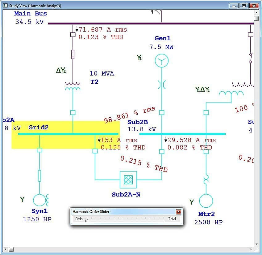
The harmonic domain is at the forefront of technology. The harmonic frequencies are all displayed in this recursive manner. This allows for the modeling of harmonic coupling, as observed in well-known synchronous machines.
The algorithm’s use of symmetrical components, phase co-ordinates, and single- or three-phase operation are just a few of the many considerations. Data entry for three-phase analysis typically requires the physical geometry of the overhead transmission lines and cables, as well as conductor details.
Using methods based on quick Fourier transforms, this information can subsequently be translated from the time domain to the frequency domain. Because of the convergence of computing techniques with speedy and typically simultaneous calculation, these data can be displayed in real time.
Time stamps from global positioning systems (GPS) enable data collected from many places to be connected. If there are enough initial monitoring points, a harmonic state estimator can be fed samples taken exactly simultaneously using the GPS time stamp, allowing it to determine the location and magnitude of harmonics entering the system, as well as harmonic voltages and currents at points that are not monitored.
Useful Video – How to perform Harmonic Analysis with ETAP
11. Earthing Study
The increasing short-circuit capability of power systems highlights the importance of properly earthing all power system equipment. The impacts of fault current on faraway, separately grounded equipment can be assessed using special software, and programs have been developed to do so in places with large electrical equipment like substations.
An earth mat of buried conductors, or electrodes (earth rods), may be used to make the connection to earth potential. The earth’s resistivity at various depths, as well as the shape and dimensions of the electrodes, their placement, and the design of an earth mat, must be described before the earth resistance can be calculated.
It is commonly assumed that all of the buried conductors and electrodes in a grid have the same potential. Different potentials can exist between grid sections due to the resistance of buried or aerial cables connecting them.
Good Video – ETAP Ground Grid System Design & Analysis
A buried link is typically thought to be able to radiate current into the ground. The fault current can be represented in a number of different ways. It is possible to set a constant current or to calculate it from the short-circuit MVA and the busbar voltage.
Faults further away from the place under study may require a more intricate fault route to be developed!
The surface potential over the damaged area can be assessed and step and touch potentials can be deduced from the analysis. Surface potentials may be shown in three dimensions, which is helpful for pinpointing trouble spots.
Suggested Guide – High voltage earthing system analysis and design for power substations and lines
High voltage earthing system analysis and design for power substations and lines
12. … And To Conclude
There are more programs out there than can be covered in this article. Those that have been brought up so far are not necessarily more important than those that have been left out. Almost any issue you may encounter with your power system has a software solution, and new solutions are continually being developed.
Verify that the software you’re using was developed to do the necessary tasks. Be careful, because some software relies on assumptions that are sufficient in most circumstances but may not be suitable for yours! The algorithm and data processing are the most crucial aspects of the application, regardless of how polished and user-friendly the interface may be.
Errors (regressions) can multiply as the complexity and interdependence of a program grows. Always double-check your replies and make sure they make sense.
Analyses will yield very different results, for instance, if the cable length is defined as 100 miles rather than 100 m.
Good to Study (PDF) – A useful guide to all practicing engineers on the subject of power system protection
A useful guide to all practicing engineers on the subject of power system protection
13. BONUS! Fault Current Calculator (XLSX) + Power Protection Analysis (PDF)
Download Fault Current Calculator (XLSX) + Power Protection Analysis (PDF) (for premium members only):
Sources:
- Practical Power Distribution for Industry by Jan de Kock and Kobus Strauss
- Analysis of transients and disturbances in electric power systems – Akihiro Ametani, Naoto Nagaoka, Yoshihiro Baba And Teruo Ohno
- Modeling and analysis of external balanced and unbalanced faults (symmetrical components) – Nasser D. Tleis BSc, MSc, PhD, CEng, FIEE
- Overcurrent protection study for a power network (solving the relay setting miss-coordination) – Ahmed Hatim Abdelbari Elniema, Ahmed Omer Mohamed Babiker And Mohamed Ali Mohamed Ibrahim at Faculty of Engineering Department of Electrical and Electronics Engineering, University Of Khartoum
Related electrical guides & articles


Edvard Csanyi
Hi, I'm an electrical engineer, programmer and founder of EEP - Electrical Engineering Portal. I worked twelve years at Schneider Electric in the position of technical support for low- and medium-voltage projects and the design of busbar trunking systems.I'm highly specialized in the design of LV/MV switchgear and low-voltage, high-power busbar trunking (<6300A) in substations, commercial buildings and industry facilities. I'm also a professional in AutoCAD programming.
Profile: Edvard Csanyi

Very Good Concept
Very good to read your book and explain how to handle 👍👍
Thank you, Wouter!