The essentials of pumping, pump speed and flow rate control that engineers MUST know

Pumping Systems and Control

Around twenty five percent of the energy that is consumed by electric motors worldwide is accounted for by pumping systems, and certain industrial facilities use anywhere from twenty-five to fifty percent of the total electrical energy available. There are significant chances to cut down on the amount of energy consumed by pumping systems through the use of intelligent design, retrofitting, and operational techniques.

The numerous pumping applications that call for variable-duty needs in particular present a significant opportunity for cost reduction. The savings typically encompass a lot more than just energy and might include things like increased performance and dependability as well as lower expenses over the product’s whole life cycle.

The majority of the currently deployed systems that call for flow control make use of bypass lines, throttling valves, or speed modifications to the pumps. The control of the pump’s speed is the most effective of these. As the speed of a pump is decreased, less energy is sent to the fluid, which in turn reduces the amount of energy that needs to be throttled or bypassed.

When discussing pumping in an appropriate manner, one must take into account not only the pump but also the “system” of pumping as a whole as well as the ways in which the components of the system interact with one another.

Evaluation and analysis based on systems is the suggested method, and this method takes into account both the supply and demand sides of the system.

Table of Contents:

1. Pumping System Hydraulic Characteristics
2. Pump Types
3. How Pump Works?
   1. Pump Characteristics
   2. Flow Rate Control
      1. Method #1 – Throttling by a Valve
      2. Method #2 – Bypassing by a Valve
      3. Method #3 – On–Off Control
      4. Method #4 – Variable Speed Control
      5. Method #5 – Running More Than One Pump
   3. Example of a Water Pump

1. Pumping System Hydraulic Characteristics

In most instances, the goal of a pumping system is either to move a liquid from its source to a required destination, such as filling a high-level reservoir, or to recirculate a liquid throughout a system, such as to transfer heat between components of the system. Both of these goals are accomplished by pumping the liquid.

It is necessary to have pressure in order to achieve the desired flow rate of the liquid, and this pressure must be sufficient to compensate for any losses that occur inside the system. There are two different kinds of losses: friction head and static head.

The square of the flow rate is proportional to the loss that occurs here. Only friction losses would be seen in a closed-loop circulating system that did not have any surfaces that were exposed to the outside air pressure.

Static and frictional heads are typically seen in combination in most systems. The benefits that can be obtained from variable speed drives (VSDs) are influenced by the ratio of static head to friction head over the working range. The presence of static head is a quality that is unique to this piece. Both the cost of the installation and the cost of pumping the liquid can typically be reduced by lowering this head whenever it is practical to do so.

In order to cut down on pumping costs, friction head losses need to be kept to a minimum. Nevertheless, even after eliminating unneeded pipe fittings and length, further reduction in friction head will require pipes with a greater diameter, which will increase the cost of installation.

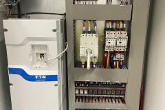
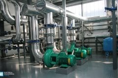
Figure 1 – VFD panel designed for a water pump application

Go back to the Contents Table ↑

2. Pump Types (Positive Displacement, Rotodynamic)

It is necessary to ensure that the pumps, motors, and controls that make up a pumping system are properly selected to fulfill the requirements of the process in order to ensure that the system runs successfully, reliably, and efficiently. Both positive displacement (PD) and rotodynamic pumps are the two primary classifications that every other type of pump falls under.

There are two primary categories that can be utilized to organize PD pumps: rotary and reciprocating. The maximum pressure that rotary pumps can normally handle is 25 bar (360 pounds per square inch [psi]). These pumps move liquid from the suction side to the discharge side by utilizing the action of spinning screws, lobes, gears, rollers, and other similar components, all of which function within of a rigid casing.

A crankshaft, camshaft, or swash-plate can be used to transform the rotating motion of the driver, which could be something as simple as an electric motor, into a reciprocating motion.

A graphic representation of the performance of a pump can be made by plotting the head against the flow rate. The rotodynamic pump has a curve that features a steady decrease in head in response to an increase in flow. On the other hand, the flow from a PD pump remains practically the same regardless of the head.

It is normal practice to draw the curve for PD pumps with the axes in the other direction; nevertheless, for the purpose of comparison, we will use a presentation that is the same for both types of pumps here.

Suggested Video – Difference Between Reciprocating and Rotary Pump

Go back to the Contents Table ↑

3. How Pump Works?

A good example of machinery that uses a lot of electricity is pumps. In light of this, it is important to focus on ways to reduce pumps’ energy consumption because doing so is both technically feasible and economically beneficial. Though the pump itself operates with a high efficiency, the rest of the pumping system (including the pipes, valves, and so on) performs poorly.

The most common form of pump is a centrifugal pump. As a general rule, they have an impeller that spins in order to transfer mechanical energy to the fluid, which is then transformed into the potential energy represented by the pressure and the kinetic energy represented by the flow rate.

See Figure 2 below.

Figure 2 – The main components of a centrifugal pump

Most of the time, the chosen pump size is too big for the job. To counteract the potential for an increase in head loss in the pipes, high-head pumps are chosen. When the demand for water and sewerage services is expected to grow in the future, pumps with a higher flow rate than they currently need are chosen.

For example, water and sewage pumping stations use many of these pumps constantly. The amount and variability of available water should be used to regulate their operation. Furthermore, many industrial pump facilities are operating inefficiently due to the use of valves to regulate flow.

Pumps are specified basically by three elements (see Figure 3):

• Flow rate Q;
• Total head H (the summation of static head H_st and dynamic head H_dyn), and
• Rotating speed N.

Figure 3 – Main components of pump specification

The pump is distinguished by its particular speed N_s. The specific speed of all impellers of the same form is constant and is computed using the relation:

where:

• N is the rotating speed (rpm.),
• Q is the flow at point of maximum efficiency (m³/min),
• H is the total head at point of maximum efficiency (m),
• K is a factor = 𝜌 g / 𝜂 (𝜌 g is the specific weight and 𝜂 is the overall pump efficiency).

The shaft power consumed by a pump is given as:

Go back to the Contents Table ↑

3.1 Pump Characteristics

The pump curve, which depicts the change of flow rate Q versus total head H, expresses the pump characteristic. Figure 4 depicts the pump characteristics for H_st = 0 and H_st > 0. The system curve in this figure depicts the fluctuation of system resistance against flow rate.

The pump operating point is determined by the intersection of the pump curve and the system curve (pump duty point).

Figure 4 – Pump characteristic (a) at H_st = 0, and (b) at H_st > 0

As illustrated in Figure 5, the power consumption of a pump remains constant when operating at its rated speed, despite variations in the flow rate. It can be seen from pump characteristic curves (both the pump curve and the system curve) that as the static head rises, the system curve rises as well since the system resistance also rises.

This may be deduced from the relationship between the two curves.

Figure 5 – Pump power consumption vs. flow rate

As a result, the operating point of the pump shifts in a direction that results in a decreasing flow rate. Figure 6 below illustrates how the rise in static head causes the flow rate to drop from Q1 to Q2 to Q3, as evidenced by the progression from Hst1 to Hst2 to Hst3.

Flow, static head, and frictional head are the three essential components that make up the pumping system. Therefore, the opportunities for saving electric power in pumps include reducing the flow and head requirements, selecting the pump type and size that is the most efficient, maintaining the pumps and all system components to avoid efficiency loss, and controlling the flow rate in an efficient manner.

Figure 6 – Pump operating point at different static heads

Go back to the Contents Table ↑

3.2 Flow Rate Control

It is common practice to observe that the daily fluid demand from a pump fluctuates. It is likely that this is the result of a number of factors, such as the passage of time, the impact of the weather, unplanned events, and the overall shift in operating conditions.

Controlling the flow rate in accordance with the required signal flow pattern is therefore an essential characteristic.

The following will provide a description of these various methods:

Method #1 – Throttling by a Valve

The process of throttling causes a rise in the resistance of the system, as depicted by the dashed line in Figure 7. Because of this, the pump’s operating point shifts, and the flow rate, rather than being Q1, becomes Q2 (Q2 is greater than Q1).

Figure 7 – Pump characteristic when throttling the output by a valve

Go back to the Contents Table ↑

Method #2 – Bypassing by a Valve

As can be seen in Figure 8, when a valve is used to go around the pump, the head pressure drops, and the operating point shifts from A to B, which results in flow rate Q3. The system curve is moving upwards, and the operating point is moving from A to C (while remaining at the same head), which results in a flow rate of Q2.

Figure 8 – Pump characteristic when bypassing by a valve

Go back to the Contents Table ↑

Method #3 – On–Off Control

When there is a clear distinction between times when a pump is needed and times when it is not needed, the pumps can be turned off during the times when they are not needed. This is referred to as the pump operating in an intermittent manner, and its characteristics are displayed in Figure 9.

Figure 9 – Pump characteristic with on-off control

The pump only uses power when in use (see Figure 10). To prevent fluid hammer effects and possibly motor overheating, this technique can be used while cycling the pump on and off for extended periods of time.

Figure 10 – Pump power consumption

Go back to the Contents Table ↑

Method #4 – Variable Speed Control

This technique is the most efficient, and it has several benefits, such as the pump running smoothly in both the low and high flow rate levels, and significant savings on electrical power costs. Changing the pump’s rotational speed alters the pump’s characteristic curve and, in turn, the flow rate.

See Figure 11 below.

Figure 11 – Pump characteristic with speed control

Go back to the Contents Table ↑

Method #5 – Running More Than One Pump

In order to cut down on the overall amount of power that is consumed, we use a different number of pumps depending on how quickly the flow rate changes. As demonstrated by the pump characteristic in Figures 12 and 13, respectively, the pumps can be linked either in parallel (to regulate the flow rate) or in series (to control the static head) in order to achieve the desired effect.

Figure 12 – Characteristics of two pumps in parallel

Figure 13 – Characteristics of two pumps in series

Go back to the Contents Table ↑

3.3 Example of a Water Pump

A water pump is working at its pump duty point when it has a flow rate of Q equal to 10 m³/m and a total head of H equal to 10 m. Figure 14 illustrates the pump characteristic of head vs flow rate. Figure 14. The flow rate is being adjusted to be 7 m³/m, which is under control.

Figure 14 – Pump characteristic at different methods of flow rate control

Where: (a) Throttle control; (b) bypassing; (c) on–off control; (d) variable speed control.

Several flow rate control systems are used, and the shaft power for each method can be computed as follows:

Assuming the factor K in above Equation equals unity, the shaft power P is given as P = Q × H(kW).

• By throttle method, as shown in Figure 14a, P = 7 × 12.7 = 88.9 ≈ 89 kW.
• Using bypassing method (Figure 14b), P = 12.4 × 6.6 = 81.84 ≈ 82 kW.
• Using on-off control (Figure 14c), where the pump is off 30% of the time,
  P = 0.7 × 10 × 10 = 70 kW.
• Using variable speed control (Figure 14d), P = 7 × 6.4 = 44.8 ≈ 45 kW.

It can be seen that variable speed control is the most effective method!

Suggested Course – Practical Course to Wiring and Setting Parameters of Variable Frequency Drives (VFDs)

Practical Course to Wiring and Setting Parameters of Variable Frequency Drives (VFDs)

Go back to the Contents Table ↑

Sources:

1. Electric Distribution Systems  By A. A. Sallam And O. P. Malik
2. Variable speed pumping – A good guide to successful applications by U.S. Department of Energy