
Estimated Study Time: 39 minutes
Relay Coordination & Selective Protection
The selected protection principle affects the operating speed of the protection, which has a significant impact on the harm caused by short circuits. The faster the protection operates, the smaller the resulting hazards, damage and the thermal stress will be. Further, the duration of the voltage dip caused by the short circuit fault will be shorter, the faster the protection operates.
 Relay Coordination and Selective Short-Circuit Protection In Transmission Networks
Thus, the disadvantage to other parts of the network due to undervoltage will be reduced to a minimum. The fast operation of the protection also reduces post-fault load peaks which, in combination with the voltage dip, increase the risk of the disturbance spreading into healthy parts of the network.
In transmission networks, any increase of the operation speed of the protection will allow the loading of the lines to be increased without increasing the risk of losing the network stability.
Thus, attention must be paid to the operating speed of the protection, which can be affected by a proper selection of the applied protection principle.
Selective short-circuit protection can be achieved in different ways, such as:
- Time-graded protection
- Time- and current-graded protection
- Time- and direction-graded protection
- Current- and impedance-graded protection
- Interlocking protection
- Differential Protection
1. Time-graded Protection
A straightforward way of obtaining selective protection is to use time grading. The principle is to grade the operating times of the relays in such a way that the relay closest to the fault spot operates first. Time-graded protection is implemented using overcurrent relays with either definite time characteristic or inverse time characteristic.
The operating time of definite time relays does not depend on the magnitude of the fault current, while the operating time of inverse time relays is shorter the higher the fault current magnitude is. The time-graded protection is best suited for radial networks.
Considering the above arguments and also taking into account, for example the short-circuit current withstand capacity of the network components, applying inverse time relays for the network short-circuit protection may be justified.
The IEC 60255-151 and BS 142 standards define four characteristic time-current curve sets for inverse time relays:
- Normal inverse
- Long-time inverse
- Very inverse
- Extremely inverse
For inverse time relays the operating time (s) can be calculated from the equation (1):
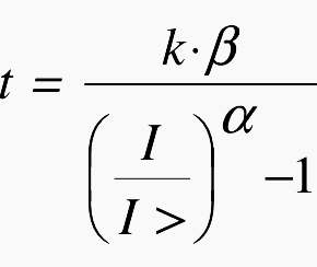
where:
- k is an adjustable time multiplier
- I is the measured phase current value
- I > is the set start (pickup) current value
- α, β are curve set-related parameters
According to the standards, the relay should start once the energizing current exceeds 1.3 times the set start current when the normal, very or extremely inverse time characteristic is used. When the long-time inverse characteristic is used the relay should start when the energizing current exceeds 1.1 times the set start current.
Table 1 The parameters α and β define the steepness of the time-current curves as follows:
| Type of characteristic | α | β |
| Normal inverse | 0.02 | 0.14 |
| Very inverse | 1.0 | 13.5 |
| Extremely inverse | 2.0 | 80.0 |
| Long-time inverse | 1.0 | 120.0 |
Figure 1 shows a time-graded protection arrangement in a radial network. In the example network, three-stage protection is implemented.
- For the low-set stage (3I>), either inverse time or definite time characteristic can be given.
- The high-set and the instantaneous stage (3I>> and 3I>>>) have definite time characteristic and their purpose is to accelerate the operation of the protection under heavy fault current conditions.
A multiple-stage protection is often required to meet with the sensitivity and operating speed requirements and to achieve a good and reliable grading of the protection, see Figure 1.
Studying and planning of time-selective protection schemes is most conveniently carried out using selectivity diagrams.
The chain of relays in the example of Figure 1 includes two relays. The selectivity diagram also includes additional information needed for the planning and operation of the protection, such as the lowest and highest fault current levels in the relaying points, maximum load current, nominal currents and short- circuit current withstand capacity of network components and the maximum limit values of possible switching inrush currents and start currents.
The selectivity diagram of Figure 1 shows that should a fault arise, for example, in the far end of the feeder (outgoing feeder 1) protected by relay 1, the fault current magnitude will be on the level indicated by [8]. This fault causes both the relay 1 and relay 2 to start (outgoing feeder 1).
Thus, the concerned feeder belongs to the protection area of the relay 1 and relay 2, providing an inherent backup protection for the feeder. Should relay 1 or its circuit breaker fail to operate, relay 2 will be allowed to operate.

The selection of the proper grading time is of essential importance for the selectivity of the protection. The grading time is the time difference between two consecutive protection stages. In heavy fault current conditions, the relay operating time must not be unnecessarily prolonged and, on the other hand, a satisfactory margin must be maintained to secure the selectivity.
In the example of Figure 1, the grading times have been defined separately for each stage. The grading time between the inverse time stages have been denoted ΔtIDMT and, correspondingly, the grading time between definite time stages has been denoted ΔtDT .
When defining the grading time, it must be noted that at lower fault current levels the prevailing load currents ΣIL of the healthy feeders during the fault must be taken into account to a certain degree. These currents are summed, for example, into the current measured by relay 2 when a fault appears on feeder 1.
When numerical relays are used, the required grading times can be calculated from Equations (2) and (2). Figure 2 shows how the grading times and the factors affecting them are formed.
For definite time relays, the grading time ΔtDT is obtained from Equation (2).
ΔtDT = 2⋅tE + tR + tCB + tM
Where:
- tE is the tolerance of the relay operating time
- tCB is the circuit breaker operating time
- tR is the relay retardation time
- tM is the safety margin
The safety margin takes into account the possible delay of the relay operation due to CT-saturation caused by the DC-component of the fault current. The length of the possible additional delay thus occurring is affected by the fault type, fault current magnitude and the ratio between the CT-accuracy limit factor and the set current value.
In theory, the delay can even be as long as the time constant of the DC-component, should the fault current just slightly exceed the set value and should the set value have been chosen just slightly below the corresponding CT-accuracy limit factor.
In practice, however, the CTs of the consecutive relays of the protection chain will saturate within a certain fault current range, which means that the operation of the relays is about equally delayed.
For this reason, a safety margin of about the length of the fundamental frequency cycle is enough.
If, however, relatively big differences in the accuracy limit factors of successive CTs in the protection chain exist, it might be justifiable to increase the safety margin in relation to the time constant of the DC-component. The safety margin is also to be increased if auxiliary relays are used in the trip circuit of the circuit breaker.
The retardation time is the time period just before the elapsing of the operation delay timer.
If the fault disappears before the starting of the retardation time, the protection relay that has been started by the fault is still able to cancel its tripping command. If the fault disappears during the retardation time just before the elapsing of the operation delay timer, the tripping command will be initiated.
The grading time ΔtIDMT for protection schemes based on inverse time relays is obtained from Equation (3):
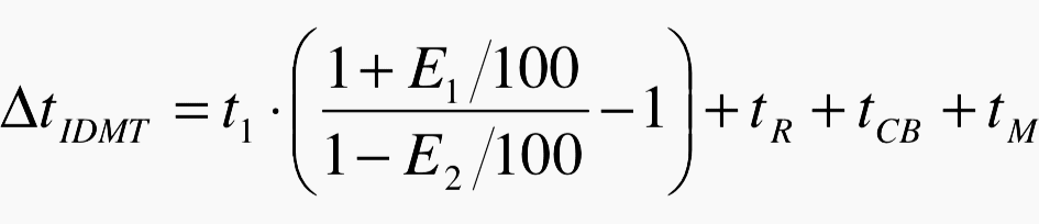
Where:
- E1 is a factor which takes into account the superimposed effect of the operating time error caused by the inaccuracy of the current measurement and the operating time tolerance in the relay located closest to the fault spot (%) *
- E2 is a factor which takes into account the superimposed effect of the operating time error caused by the inaccuracy of the current measurement and the operating time tolerance in the relay located next in the protection chain (%) *
- tCB is the circuit breaker operating time
- tR is the retardation time
- tM is the safety margin
- t1 is the calculated operating time of the relay closest to the fault spot *
* Corresponds to the current value with which the grading time is determined, Figure 2.
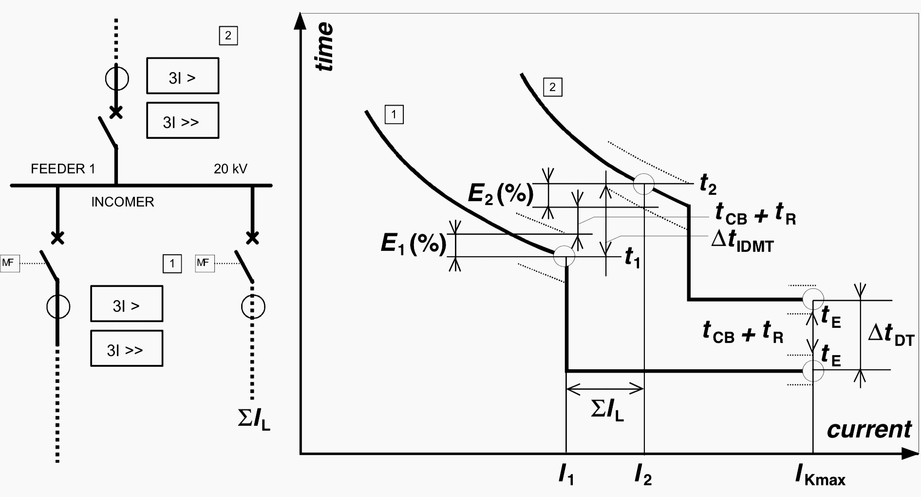
- I1 , I2 = current values with which the grading time between the low-set stages (3I>) is determined,
- Ikmax = maximum short-circuit current.
- For other notations, see Equations (2) and (3).
The tolerance values of the operating times are standardized, Table 2:
Table 2 – Limit values, according to the BS 142 standard, of the operating times expressed as a percentage. E = accuracy class index
| I/I> | Normal inverse | Very inverse | Extremely inverse | Long time inverse |
| 2 | 2.22×E | 2.34×E | 2.44×E | 2.34×E |
| 5 | 1.13×E | 1.26×E | 1.48×E | 1.26×E |
| 7 | – | – | – | 1.00×E |
| 10 | 1.01×E | 1.01×E | 1.02×E | – |
| 20 | 1.00×E | 1.00×E | 1.00×E | – |
Furthermore, the effect of the current measuring inaccuracy on the operating time of the inverse time protection must be observed. The effect can be evaluated using Equation (1) by giving values to the phase current according to the measuring inaccuracy used.
The measuring inaccuracy is affected not only by the relay type but also by the accuracy of the measurement transformers. By adding the percentage of the operating time inaccuracies thus obtained to the values of Table 2 , the values of the factors E1 and E2 can be found.
Example of the determination of the grading time ΔtDT
The grading time between the high-set stages of the numerical protection relays in Figure 1 is determined using the Equation (2):
- 2 times the tolerance of the operating time: 2 × 25 ms
- Circuit breaker operating time: 50 ms
- Retardation time: 30 ms
- Safety margin: 20 ms
- Total: 150 ms
The safety margin has been given the smallest possible value, and so the grading time ΔtDT =150 ms can be chosen, see Figure 1.
Example of the determination of the grading time ΔtIDMT
The grading time between the low-set stages of the numerical protection relays in Figure 1 is determined using Equation (3):
Current values with which the grading time is determined:
- Relay 1: I1 = 1200 A ≈ 4.0 times the current setting of the stage
- Relay 2: I2 = 1700 A ≈ 2.4 times the current setting of the stage
The selected curve type is normal inverse and the accuracy class E which equals 5%.
The effect of the current measuring inaccuracy on the operating times in per cent from the calculated operating times t1 and t2 is determined using Equation (1), and when the joint current measuring inaccuracy of the relay and the measurement transformer is expected to be ±3%, Table 3 and Table 4.
It must also be noted that the operating time error thus arising is independent of the setting of the time multiplier k of the inverse time curve.
Table 3 – The effect of the current measuring inaccuracy on the operating times in relation to the calculated operating times t1 of relay 1 for the current I1
| I1 (× I>) | Current measurement error (%) | Operating time error (t – t1) / t1 × 100 (%) |
| 4.0 | +3 | -2 |
| 4.0 | -3 | +2 |
Table 4 – The effect of the current measuring inaccuracy on the operating times in relation to the calculated operating times t2 of relay 2 for the current I2
| I2 (× I>) | Current measurement error (%) | Operating time error (t – t2) / t2 × 100 (%) |
| 2.4 | +3 | -3 |
| 2.4 | -3 | +3 |
The factors E1 and E2 are calculated as the sum of the absolute values of the errors:
- Relay 1: E1 = 8%
- Relay 2: E2 = 14%
By inserting factors E1 and E2 into Equation (3) and by observing that the calculated operating time t1 of relay 1 is 1000 ms at 1200 A (4 × the set current), the required grading time can be calculated as follows:
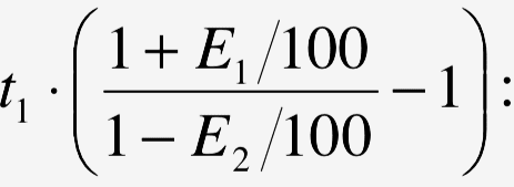 | 260 ms |
| CB operating time: | 50 ms |
| Retardation time: | 30 ms |
| Safety margin: | 20 ms |
| Total: | 360 ms |
According to this, the grading time ΔtIDMT should be given a value of at least 360 ms, Figure 1.
Underimpedance relays
The time-graded protection can also be implemented with definite time underimpedance relays. The relay measures the phase currents and phase-to-phase or phase-to-earth voltages. Based on these values, it determines the apparent impedance seen from the relay location.
The relay operates if the measured impedance falls below the set start value. The set start value determines the so-called reach of the relay, which defines at which distance faults seen from the relaying point can still be detected. Owing to the measuring principle, the advantage of the impedance relay is that its operation is independent of the short-circuit power of the incoming network.
The reach and the operating time of the relay are unchanged even if the source impedance changes, for example, when the network configuration is altered.
Thus the relay operates reliably even though the short-circuit current would be particularly low.
If the protection of the outgoing lines from the power plant is also based on the impedance-measuring principle, selectivity between the relays can be easily obtained. The aforementioned salient principles of time grading also apply to underimpedance protection.
2. Time- and Current-graded Protection
Time- and current-graded protection can be used in cases where the fault current magnitudes in faults occurring in front of and behind the relaying point are different. Due to the different fault current levels using inverse time relays but also multi-stage definite time relays, different operating times can be obtained in either direction. In this way the requested time grading can be obtained and the operating time requirements can be fulfilled.
Figure 3 shows an example time- and current-graded overcurrent protection application.
The study of the time grading towards one particular generator feeder is straightforward if the operating characteristic of the protection of the other generator feeders are combined in a single operating characteristic of a so-called equivalent generator feeder.
This is obtained by multiplying the current values of the relay operating characteristic of a single generator by the number of generators in use at any time, operating characteristic 3G , Figure 3.
It can clearly be seen that in this way a reliable time-grading is obtained between the generator feeders also in cases where the fault current fed by the network is particularly low or if one generator is out of operation.
The same method of study can be applied for planning the time-grading between the protection relays of the block transformer and the generator feeders for faults occurring in the network side.
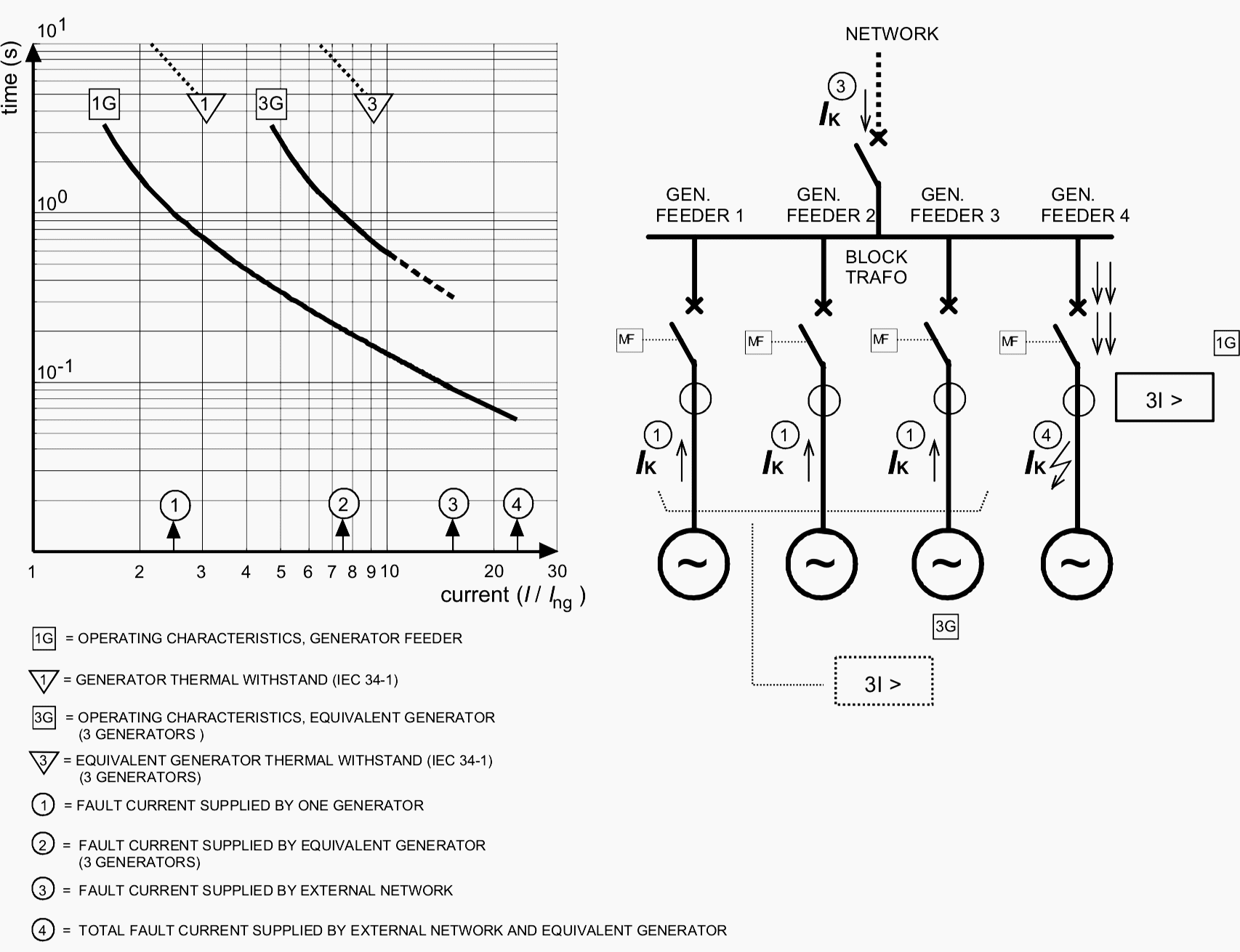
Where: Ing is rated current of a single generator.
In this planning, special attention must be paid to the number of generators in operation and its effect on the the selectivity. Should machines be taken out of operation, the time-grading towards the network can be endangered if the settings of the protection relays of the block transformer are not adapted to the operating conditions at any time.
The protection practice described can also be used in the overcurrent protection of ring and meshed networks. Another area of application is the earth fault protection of effectively earthed ring and meshed networks.
3. Time- and direction-graded protection
In ring and meshed networks, the selectivity of the protection can be based on directional overcurrent relays.
Directional relays are needed as different operating times are required depending on the location of the fault, that is, if the fault spot is in front of the relaying point on the feeder or behind the relaying point, for example, on the incoming feeder or on the busbar system.
Typical applications based on directional protection are shown in Figure 4.

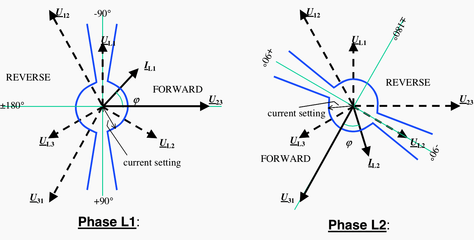
Various principles are used for determining the direction of the fault current. The most conventional way is to determine the direction phase-specifically so that the current phasor of each faulty phase is compared to the phasor of the opposite phase-to-phase voltage, for example, the direction of the phase current phasor IL1 is compared to the direction of the phasor U23.
The relay operates if one or more of the direction comparisons show that the fault is located in the forward or reverse direction with regard to the set relay operating direction.
An example operating characteristic formed in this way is shown in Figure 5.
Another way of determining the direction is first to indentify the faulty phases on the basis of the starts of the phase-specific overcurrent functions and then compare the difference between these current phasors to the difference between the other two phase-to-phase voltages, for example, the direction of the phasor IL1 − IL2 is compared to the direction of the phasor U23 − U31.
Alternatively, the phasor IL1 − IL2 can also be compared to the direction of the corresponding faulty phase-to-phase phasor U12 , or to the corresponding positive-sequence voltage U1 ,which must be suitably rotated according to the fault type in question.
The said direction determination methods need to be supported by a voltage memory which stores the phasors of the pre-fault voltages. The relay uses the stored information for determination of the fault current direction in cases where the voltages are too low to be measured, that is, close-in short circuits.
However, the advantage of this method is that the phase order of the power system has no impact on the direction determination.
The protection of ring and meshed networks can also be carried out using directional definite time underimpedance or distance relays. These relays are frequently used for the protection of transmission and sub-transmission networks, meshed or ring-operated distribution networks or weak radial networks.
The advantages of the use of distance relays are the same as for the underimpedance relays in general, and the general time-grading principles also apply in this protection concept.
To achieve a good and reliable selectivity and to fulfill the operating speed requirements as well as possible, it is typically necessary to implement multiple directional underimpedance stages. The reach of these stages defines the zones of protection toward the desired operating direction, which can be either forward of reverse.
An example of this can be seen in Figure 6, where multiple-stage numerical distance relay units are applied to the short-circuit protection of a sub-transmission network. The figure also shows the principal reaches of the different zones of the example relay unit.
The zones Z1, Z2 and Z3 are set in the forward direction, that is, toward the protected line and the zone Z4 in the reverse direction.

Where: MV = distribution voltage
Zone Z1 is underreaching the remote end station, making it possible to apply minimum operating times.
Zone Z2 is slightly overreaching the remote end, which means that the time coordination with zone Z1 of the successive line is required. Therefore the operating time is delayed as much as the grading margin requires.
Zone Z3 operates as an overreaching backup protection and the operating time must be selected so that it coordinates with the protection in the forward direction in all conditions.
Zone Z4 operates as an overreaching backup protection in the reverse direction, and the reach of this zone is selected so that it can detect faults even on the MV-side of the transformers. The operating time is selected accordingly. The main purpose of the zone Z4 is to operate as a backup protection for the transformers.
The main advantage of using distance relays in this example is that all faults occurring in the sub-transmission network can be cleared by the zones Z1 or Z2 in less than 0.2 seconds. Also possible fault current infeed from the distribution network side due to distributed generation, for example, does not affect the selectivity of the protection.
4. Current- and Impedance-graded Protection
In certain cases, protection principle based on current and impedance grading can be used to essentially accelerate the operation of the protection in faults arising close to the relaying point. The protection is implemented by using one directional or non-directional stage of the overcurrent or underimpedance relay.
The intention is to set the start current of the overcurrent stage so high that when a fault arises in front of the next relay in the protection chain, the concerned stage will not operate and no time-grading is needed. Correspondingly, when an underimpedance stage is used, the reach should be set low enough to obtain the corresponding function.
For example, in Figure 6 the zone Z1 operates according to this principle.
Therefore, a normal time-graded protection arrangement should always be incorporated in parallel with the protection based on current or impedance grading.
When the settings of a current-graded protection arrangement are determined, the behavior of the relay type used in unsymmetrical faults must be taken into account, that is, does the DC-component of the fault current possibly cause a so-called transient overreach kDC (%), which is defined as:
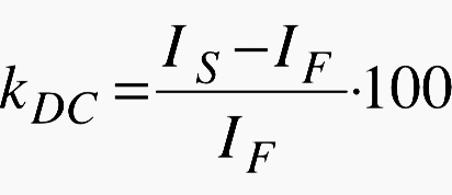
where:
- IS is the RMS-value of the steady-state phase current at which the protection operates, that is, the set current.
- IF is the RMS-value of the steady-state phase current onto which a superimposed full DC-component causes the protection to operate at the set current IS
The primary value of the set start current of the current-graded overcurrent stage should be higher than or equal to ICS:
ICS = km × (1 + kDC / 100) × IK
Where:
- km is a safety factor which takes into account the inaccuracy of the fault current calculation and the errors of the measurement transformers and the relay. A typical value equals 1.2.
- IK is the maximum fault current, which is calculated in the location of the successive/next relay in the protection chain
Especially the application of the current grading requires a sufficiently low source impedance ratio (SIR), Equation (6) below, at the relaying point. In the current-graded protection, this ensures that the fault current difference in the beginning and the end of the protected feeder, or in the HV- and the MV-side of the protected transformer, is high enough to enable suitable settings to be found for the protection.
The higher the SIR-value, the shorter the reach of the protection on the protected feeder will be.
SIR = |ZS| / |ZL|
Where:
- ZS is the impedance of the incoming network, that is, the source impedance as seen from the relaying point
- ZL is the impedance of the protected feeder as seen from the relaying point
A high SIR-value may also limit the use of the impedance-graded protection concept because in such a case the magnitudes of the currents and voltages measured by the protection at the end of the zone and in the immediate vicinity may be so close to each other that measuring errors may cause a false operation of the protection.
5. Interlocking-based Protection
The purpose of interlocking-based protection is to accelerate the operation of the protection. The concept is especially suited for busbar protection, but it can also be implemented for the protection of short outgoing and incoming feeders and the transformer MV-side.
In the example of Figure 7, the protected object is a busbar system, the bus tie circuit breaker of which is normally open. When a fault arises on the feeder, the overcurrent relays of both the incoming and outgoing feeders start.
The overcurrent relay of the faulty feeder sends an interlocking signal that blocks the operation of the 3I>>>-stage of the incoming feeder relay and trips the circuit breaker after the set time delay. When the fault appears within the area of protection, that is, on the busbar, no interlocking signals will be generated and the 3I>>>-stage of the incoming feeder relay trips the circuit breaker after the set time delay, which is shorter than what would be required in the time-graded solution in the corresponding situation.
When also the bus tie circuit breaker is incorporated in the interlocking chain, the protection operates selectively even if the bus tie circuit breaker were closed.
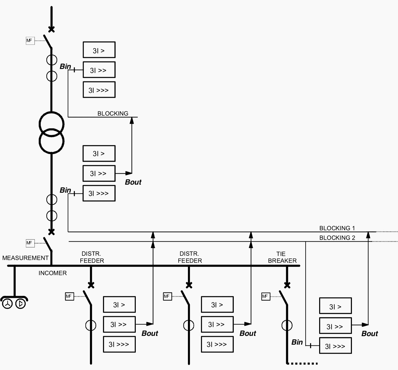
Where:
- Bout = transmitted interlocking signal,
- Bin = received interlocking signal, which blocks the operation of the concerned overcurrent stage.
The interlocking-based protection concept is best suited for use in radial networks, where the short-circuit currents are considerably higher than the load currents. In this case, a current setting value can easily be found for the overcurrent stage that issues the interlocking signal.
For a reliable and selective operation, the overcurrent stage to be interlocked must be slightly delayed. In the example of Figure 7, the 3I>>>-stage of the incoming feeder relay is used for this purpose. The required delay depends on the features of the relay type applied, the accuracy limit factors of the CTs and the implementation of the interlocking channel.
The required operating delay can be estimated by observing the following:
- Start time of the overcurrent stage issuing the interlocking signal. This starting time includes both the start delay of the stage and the inherent delay of the binary output of the relay (typically <40 ms)
- Retardation time of the overcurrent stage to be blocked including the response time of the binary input of the relay (typically < 30 ms)
- Safety margin that, for example, takes into account the effect of the possible saturation of the current transformers (typically 1 to 2 cycles)
By summing the delay times mentioned, the shortest possible time setting for the overcurrent stage to be blocked is obtained. Typically this time is about 100 ms, provided that no auxiliary relays are incorporated in the blocking circuit.
The interlocking protection principle can also be applied in ring or meshed networks, in which case directional overcurrent relays or distance relays are to be used.
Because the protection areas of the interlocking-based protection concept are not overlapping and because they do not reach into the protection area of the next relays in the protection chain, a parallel time-graded protection system must always be used.
In Figure 7 this time-graded protection is implemented with one to three stages depending on the relay location.
Reference // Distribution Automation Handbook – Relay Coordination by ABB
Related electrical guides & articles


Edvard Csanyi
Hi, I'm an electrical engineer, programmer and founder of EEP - Electrical Engineering Portal. I worked twelve years at Schneider Electric in the position of technical support for low- and medium-voltage projects and the design of busbar trunking systems.I'm highly specialized in the design of LV/MV switchgear and low-voltage, high-power busbar trunking (<6300A) in substations, commercial buildings and industry facilities. I'm also a professional in AutoCAD programming.
Profile: Edvard Csanyi

Honestly this is what the senior engineers did in the simulation before we energized 13MVA & 12MVA transformer’s today. Thou I didn’t understand the scenarios well. Thanks 🙏👍 a lot, you’ve helped me alert. I’m so sorry it’s quite expensive to subscribe to your premium plan cause of Dollar to Naira exchange rate here.
AoA,
A great achievement ,felicitations to your honor and your team. With Best Regards :Engr Muhammad Abdullah Khalid Seyal,PhD Scholar
Can you arrange more examples on time grading.And also I am not understand that E1 and E2.please send to my mail id [email protected].
This article overall good.
Great service to engineering community
fantastic info, great details thanks, broad knowledge.
Very informative and simple to understand. Keep up the great work.