
Estimated Study Time: 19 minutes
New MV/LV distribution substation
Designing a new MV/LV distribution substation is somewhat complicated and involves a lot of factors you must take care of. This technical article will try to present the essential steps in starting the design process. The beginning is always the hardest part, but once you learn the principles, it will be much easier for the next substations.
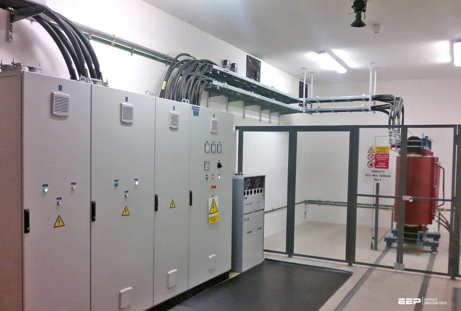 The story of designing the electrical part of MV/LV power substation (photo credit: Elektromont servis Brno, spol. s r.o.)
Generally, the article is based on two main parts. The first part is dedicated to the estimation of load you will have in your project (small factory as an example). The second part in more complicated and involves the various network calculations of short circuit and protection coordination.
Note that many people should be involved in obtaining all the necessary information for the project. A good start would be contacting the power supply utility personnel for sizing of the equipment, calibration of protection devices, the design and verification of the earthing system regarding the supply. Then, collecting “true” information about loads could be a painful job, etc.
Ok, let’s dive into estimations and calculations!
- Estimate of the power (supplied to a small industrial factory)
- Calculation of short circuit and coordination of protections
1. Estimate of the power supplied to a small industrial factory
Let’s take a small industrial plant as an example (Figure 1). Production involves a stabilized thermal cycle in the furnace for which reason a total black-out is not possible. The plant is also located in a densely populated area.

The starting point for the design is the estimation of the consumption of the various users. If in assessing the required power you were to consider the sum of the rated power of all equipment and users you would get a value that is certainly excessive, for two reasons:
- Some equipment might not be used at its full power
- The equipment will not all be work at the same time
This is taken into account with two coefficients: the utilization factor Ku and the contemporaneity factor Kc.
Therefore one has to estimate the actual load by using factors derived statistically on homogeneous categories of installations as proposed by CEI Guide 99-4, Annex E, presented below.
Table 1 – Load estimation by using factors derived statistically on homogeneous categories of installations
| Type of system | Type of environment | ||||
| Individual housing units | Civil buildings for housing | Offices, shops, warehouses, departments | Hotels, hospitals | Medium and high power industrial plants | |
| Lighting | 66% of the installed power | 75% of the installed power | 90% of the installed power | 75% of the installed power | 90% of the installed power |
| Heating | 100% of the power of the equipment up to 10A + 50% of the remainder | 100% of the biggest user + 50% of the remainder | 100% of the biggest user + 75% of the remainder | 100% of the biggest user + 80% of the second + 60% of the remainder | 100% of the biggest user + 75% of the remainder |
| Kitchens | 100% of the power of the equipment up to 10A + 30% of the equipment over 10A permanently connected | 100% of the biggest user + 80% of the second + 60% of the remainder | – | 100% of the biggest user + 80% of the second + 60% of the remainder | – |
| Motors (with the exclusion of lifts, elevators, cranes, etc.) | – | – | 100% of the biggest motor + 80% of the second motor + 60% of the remainder | 100% of the biggest motor + 80% of the second motor + 60% of the remainder | To be considered on a case by case basis |
| Water heaters | No contemporaneity is allowed | ||||
| Socket outlets | 100% of the biggest user + 25% of the remainder | 100% of the biggest user + 25% of the remainder | 100% of the biggest user + 40% of the remainder | 100% of the biggest user + 75% of the rooms + 25% of the remainder | 25% of the user installed |
Alternatively you can use table 101 of the Standard EN 61439-2:
Table 2 – Values of assumed loading
| Type of load | Assumed loading factor |
| Distribution: 2 and 3 circuits | 0.9 |
| Distribution: 4 and 5 circuits | 0.8 |
| Distribution: 6 and 9 circuits | 0.7 |
| Distribution: 10 and more circuits | 0.5 |
| Electric actuator | 0.2 |
| Motors ≤ 100 kW | 0.8 |
| Motors > 100 KW | 1.0 |
In the example provided, the power used on the main LV switchgear is 732 kVA. Considering the values of the rated power of the transformers available commercially, it can be assumed that two transformers 400 kVA transformers will be installed. Apparently, this assumption would be resulting in a more expensive solution than that with only one 800 kVA transformer.
Nevertheless, that can be justified by the need to have a greater continuity of service in case of failures or maintenance.
The other features of the substation are:
- The substation is powered by a buried cable
- The transformers are closed in parallel on the secondary so as to guarantee the power supply of the LV installation by both of them
- The size of the internal MV network is less than 400 m
Table 3 – Power consumption per departments

2. Calculation of short circuit and coordination of protections
2.1 Theory behind calculation of the short-circuit current
To deal with the theory of calculation of short-circuit currents we will refer to the Standard IEC 60909-0 “Short-circuit currents in three-phase AC systems – Part 0: Calculation of currents”. With reference to the electrical network schematized in Figure 2, a short-circuit is assumed on the load terminals.
The change from impedance values Z1 referring to a higher voltage (U1) to the values Z2, referring to a lower voltage (U2), takes place using the transformation ratio K = U1/U2 according to the following relationship:

The structure of the electrical network in question can be represented through elements in series. In this way an equivalent circuit is obtained like that shown in the following Figure 3 which makes it possible to calculate the equivalent impedance seen from the fault point.
An equivalent voltage source (Ueq) is positioned at the point of the short circuit with the value:
Ueq = c × Un / √3
The factor “c” depends on the system voltage and takes into account the influence of the loads and of the variation in mains voltage. The following is the table taken from Standard IEC 60909-0.
Table 4 – Voltage factor c for the calculation of max. and min. short-circuit currents
| Nominal voltage Un | Voltage factor c for the calculation of: | |
| Maximum short-circuit currents Cmax(1) | Minimum short-circuit currents Cmin | |
| Low voltage 100 V to 1000V (IEC 60038, table I) | 1.05(3) 1.10(4) | 0.95 |
| Medium voltage > 1kV to 35 kV (IEC 60038, table III) | 1.10 AM | 1.00 |
| High voltage(2) > 35 kV (IEC 60038, table IV) | ||
Where:
- Cmax Un should not exceed the highest voltage Um for equipment of power systems.
- If no nominal voltage is defined CmaxUn = Um or CminUn = 0.90×Um should be applied
- For low-voltage systems with a tolerance of + 6%, for example systems renamed from 380 V to 400 V
- For low-voltage systems with a tolerance of + 10%
2.2 Power supply network
In most cases, the installation will be supplied by a medium voltage distribution network, for which it is quite easy to obtain the value of the supply voltage UnQ and the initial short-circuit current I”kQ.
On the basis of these data and of a correction coefficient for the change in voltage caused by the short-circuit it is possible to determine the short-circuit direct impedance of the network with the following formula:
ZQ = c × UnQ /( √3 × I”kQ)
For the calculation of the network resistance and reactance parameters, if a precise value for value for RQ is not available, the following approximate formulas can be used:
XQ = 0.995 × ZQ
RQ = 0.1 × XQ
2.3 Transformer
The impedance of the machine can be calculated using the rated parameters of the machine itself (rated voltage UrT; apparent power SrT; short circuit voltage at the rated current in percent ukr) using the following formula:
ZT = (ukr / 100%) (UrT2 / SrT)
The resistive component can be determined by knowing the value of the total losses. PkrT referring to the rated current according to the following relationship:
RT = PkrT / (3 × IrT2)
The reactive component can be determined with the classic relationship:
XT = √(ZT2 – RT2)
2.4 Cables
The impedance value of these connection elements depends on various factors (technical, constructive, temperature, etc.) that condition the linear resistance R’L and the linear reactance X’L. These two parameters expressed per unit of length are provided by the manufacturer of the cable.
R’Lθ = [1 + α (θ – 20)] × R’L20
where α is the temperature coefficient that depends on the type of material (for copper, aluminum and aluminum alloys 4×10⁻³ holds true with good approximation). Therefore, in very simple terms we have:
RL= L × R’L and XL= L × X’L
with L the length of the cable line.
2.5 Calculation of the short-circuit current
The definition of the short-circuit resistance and reactance values of the main elements forming a circuit allow the short circuit currents in the installation to be calculated.
With reference to Figure 4, with the method of reducing elements in series the following values are determined:
- The total short-circuit resistance value R = ∑Ri
- The total short-circuit reactance value X = ∑Xi
Once the two preceding parameters are known, it is possible to determine the total short-circuit direct impedance Z:
Z = √(R2 + X2)
Once the equivalent impedance seen from the fault point has been determined, one can proceed with the calculation of the symmetrical three-phase initial short-circuit current:
I”k3 = c × Un / √3 Z

The three-phase short circuit is generally considered as the fault which causes the highest currents (except in particular conditions).
In the absence of rotary machines, or when their action is diminished, it also represents the permanent short-circuit current and is the value taken as a reference to determine the breaking capacity of the protection device.
2.6 Calculation of the contribution of motors
In the event of a short circuit, the motor starts to function as a generator and powers the fault for a limited time corresponding to the time required to eliminate the energy that has been stored in the magnetic circuit of the motor.
In low voltage, the Standard IEC 60909-0 provides the minimum indications for which the phenomenon must be taken into account, it will be:
∑IrM < 0.01 × I”k
where:
- ∑IrM represents the sum of the rated currents of the motors connected directly to the network where the short circuit occurs.
- I”k is the initial three-phase short-circuit current determined without contribution of motors.
If it has to be taken into account, the impedance of the motors may be calculated using the formula:

where:
- Urm is the rated voltage of the motor
- IrM is the rated current of the motor
- SrM is the rated apparent power of the motor (SrM = PrM/(ηrM cosφrM)
- ILR/IrM is the ratio between the locked rotor current and the rated current of the motor.
Finally, for groups of low voltage motors connected via cables we can, with good approximation, use the relationship:
RM/XM = 0.42 with XM = 0.922 ZM
2.7 Calculation of the peak current
The short circuit current I”k can be considered to consist of two components:
- A symmetrical component is with sinusoidal wave form and in fact symmetrical in relation to the horizontal time axis.
- A unidirectional component iu with exponential trend due to the presence of an inductive component.
This component is characterized by a time constant τ= L/R (“R” indicates the resistance and “L” indicates the inductance of the circuit upstream of the failure point) and is extinguished after 3-6 times τ.
During the transitional period, the unidirectional component makes the short-circuit current asymmetric, characterized by a maximum value, referred to as the peak value, which is higher than what it would be with a purely sinusoidal magnitude.
In general we can say that, considering the effective value of the symmetrical component of the short-circuit current Ik, the value of the first peak current may vary from:
√2 I”k to 2√2 I”k
After the transitional period, the short-circuit current becomes practically symmetrical. An example of the current trend is shown in the following Figure 5.

The Standard IEC 60909-0 provides useful indications for calculating the peak current. In particular, it indicates the following relationship:
ip = k × √2 × I”k
where the value of k can be evaluated with the following approximate formula:
k = 1.02 + 0.98 × e-3R/X
or through the following charts that show the value of “k” as a function of the parameter “R/X” or “X/R” (see Figure 6).

2.8 Sizing and coordination of the protections
Knowledge of certain parameters is fundamental for sizing the installation. Calculations and the study of protection coordination has been published earlier in several other technical articles, so this won’t be covered here.
Please refer to the following articles:
Properly engineered and installed selective coordination between LV circuit breakers
Proper selection and overcurrent coordination of LV/MV protective devices
Coordination problems in electrical networks that lead to nuisance CB tripping
Sources:
- Technical guide The MV/LV transformer substations (passive users) by ABB
- Schneider Electric Low voltage expert guides no. 5 – Coordination of LV protection devices
Related electrical guides & articles


Edvard Csanyi
Hi, I'm an electrical engineer, programmer and founder of EEP - Electrical Engineering Portal. I worked twelve years at Schneider Electric in the position of technical support for low- and medium-voltage projects and the design of busbar trunking systems.I'm highly specialized in the design of LV/MV switchgear and low-voltage, high-power busbar trunking (<6300A) in substations, commercial buildings and industry facilities. I'm also a professional in AutoCAD programming.
Profile: Edvard Csanyi

Can you please kindly discuss and explain in details regarding ELCBs. Especially the Current ELCB. Thank you..
Great article!
Could you clarify what K2 symbolises in figure 2?
After looking in IEC 60909-0 I am unsure whether it represents negative sequence impedance correction factor or a line-to-line short circuit?
Thanks in advance!
Sir,
Can we add a Bus coupler at Figure-1 ?
Regards.
Thank you Shashi.
Awesome Writing! Have been always a great fan of your great articles.
Amazing