The essentials of overcurrent protection you are not allowed to forget (types and principles)

Back to how it works…

Relay protection is nowadays completely digitalized and very sophisticated; there is no doubt about that. But, do electrical engineers really understand what they do when setting parameters and navigate through endless menus on a relay? Most engineers do know, of course, but the memory naturally fades over time, and it’s a good thing to refresh the basics you learned many years ago.

Overcurrent protection is often confused with overload protection which is related to the thermal capability of circuits. Overcurrent protection is primarily provided for the correct clearance of faults. Very often, engineers adopt settings that make some compromise in order to cover both of these protection objectives.

Overcurrent protection in low- and medium voltage networks can be achieved by the use of fuses, by direct-acting trip mechanisms on circuit breakers or by protection relays.

This technical article covers the essentials of overcurrent protection principles and rules.

1. Types of overcurrent system
   1. Overcurrent and earth-fault protection systems
   2. Grading of current settings
   3. Grading of time settings: the definite-time system
   4. Grading by both time and current: inverse-time overcurrent systems
      1. Fuses
      2. Delayed action a.c. trip coils
      3. Fuse shunted a.c. trip coils
      4. Inverse-time relays
2. Selection of overcurrent protection settings
   1. Data needed for system analysis

1. Types of overcurrent system

Where a source of electrical energy feeds directly to a single load, a little complication in the circuit protection is required beyond the provision of an overcurrent device that is suitable in operating characteristics for the load in question, i.e. appropriate current setting possibly with a time-lag to permit harmless short time overloads to be supplied.

Development of the power system to one such as is shown in Figure 1, in which the power source A feeds through a number of substations B, C, D, and E, from each of the busbars of which load is taken necessitates a more selective treatment.

Circuit breakers are installed at the feeding end of each line section and a graded scheme of protection is applied.

Figure 1 – Radial distribution system

Go back to Contents Table ↑

1.1 Overcurrent and earth-fault protection systems

Overcurrent protection involves the inclusion of a suitable device in each phase since the object is to detect faults that may affect only one or two phases. Where relays are used, they will usually be energized via current-transformers, which latter are included in the above statement.

Typical arrangements are shown in Figure 2 below.

The magnitude of an inter-phase fault current will normally be governed by the known impedances of the power plant and transmission lines; such currents are usually large.

Figure 2 – Types of overcurrent protection

Phase-to-earth fault current may be limited also by such features as:

1. the method of earthing the system neutral
2. the characteristics of certain types of plant, e.g. faults on delta-connected transformer windings
3. resistance in the earth path.

In consequence, earth-fault current may be of low or moderate value and also often rather uncertain in magnitude particularly on account of item (c) above.

Three current transformers, one in each phase, have their secondary windings connected in parallel, and the group connected to a protective device, either a circuit-breaker tripping coil or a relay.

Figure 3 – Residual circuit and earth-fault relay

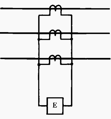
With normal load current, the output of such a group is zero, and this is also the case with a system phase-to-phase short circuit. Only when current flows to earth is there a residual component that will then energize the protective device. Since the protection is not energized by a three-phase load current, the setting can be low, giving the desired sensitive response to earth-fault current.

Phase-fault and earth-fault protection can be combined, as shown in Figure 4. The protection scheme, involving equipment at a series of substations, can be graded in various ways, the significance of which is examined below.

Figure 4 – Combined phase and earth-fault protection

Go back to Contents Table ↑

1.2 Grading of current settings

If protection is given to the system shown in Figure 1 by simple instantaneous tripping devices, set so that those furthest from the power source operate with the lowest current values and progressively higher settings apply to each stage back towards the source, then if the current were to increase through the range of settings, the device with the lowest setting of those affected would operate first and disconnect the overload at the nearest point.

Faults, however, rarely occur in this way: a short circuit on the system will immediately establish a large current of many times the trip settings likely to be adopted and would cause all the tripping devices to operate simultaneously.

One might attempt to set the circuit breaker trips to just operate with the expected fault current at the end of the associated feeder section, but this would not be successful since:

Reason #1 – It is not practicable to distinguish in magnitude between faults at F₁ and F₂, since these two points may, in the limit, be separated by no more than the path through the circuit breaker. The fault current at the alternative fault locations will then differ by only an insignificant amount (e.g. 0.1% or less) necessitating an unrealistic setting accuracy.

Reason #2 – In the diagram, the fault current at F₁ is given as 8800 A when the source busbar fault rating is 250MVA. In practice the source fault power may vary over a range of almost 2:1 by, for example, the switching out of one of two supply transformers; in some cases a bigger range is possible.

A minimum source power of 130 MVA may be assumed for illustration in this example, for which the corresponding fault current at F₁ would be only 5400 A and for a fault close up to Station A the current would be 6850 A. A trip set at 8800 A would therefore not protect any of the relevant cable under the reduced infeed conditions.

It is, therefore, clear that discrimination by current setting is not in general feasible.

Figure 5 – Radial system with variation in fault current due to feeder impedance

A single exception to the above deduction occurs when there is a lumped impedance in the system. Where, as in the last section of Figure 5, the line feeds a transformer directly, without other interconnections, there will be a significant difference in the fault current flowing in the feeder for faults, respectively, on the primary and on the secondary side of the transformer.

In many cases, it is possible to choose a current setting that will inhibit operation for all secondary-side faults, while ensuring operation for all primary side faults under all anticipated infeed conditions. The transformer is not necessarily adequately protected by such high set protection.

In special cases, instantaneous relays with high settings are used as a supplementary feature to other protection systems.

Go back to Contents Table ↑

1.3 Grading of time settings: the definite-time system

The problem discussed in the preceding Section is resolved by arranging for the equipment which trips the circuit breaker most remote from the power source, to operate in the shortest time, each successive circuit breaker back towards the supply station being tripped in progressively longer times; the time interval between any two adjacent circuit breakers is known as the ‘grading margin‘.

In this arrangement, instantaneous overcurrent relays are used in the role of starters or fault detectors. They could, in principle, have identical settings but are better with graded current settings increasing towards the supply station.

These fault-detector relays initiate the operation of d.c. definite time relays, which are set to provide the required time grading. This system is therefore known as ‘definite-time overcurrent protection‘.

Figure 1 – Radial distribution system

Referring to the radial system of Figure 1, busbar E feeds separate circuits through fuses. A relay at D might have an instantaneous operation with a high current setting which will not permit operation with a fault at E. Alternatively, if this is not feasible on account of the range of possible current, a lower current setting, but one above the maximum load current, may be used with a time setting chosen to discriminate with the fuse blowing.

Usually, a time lag of 0.2 s is sufficient, although it is desirable to check the suitability of this value for a fault current equivalent to the overcurrent element setting.

The relay at C may be set to operate in 0-5 s longer than that at D, i.e. in 0.7 s, and those at B and A will be progressively slower by the same amount, giving an operating time for relay A of 1.7 s.

The only disadvantage with this method of discrimination is that faults close to the power source, which will cause the largest fault current is cleared in the longest time.

At substations B, C, and D, loads are connected through transformers. The time setting on these circuits is selected in the same way as that at D on the feed to E and should never be greater than that on the outgoing feeder from the same busbars.

Go back to Contents Table ↑

1.4 Grading by both time and current: inverse-time overcurrent systems

The disadvantage of the definite time system mentioned above is reduced by the use of protective devices with an inverse time-current characteristic in a graded system. Figure 6 shows two time-current curves in which the operating time is in inverse ratio to the excess of current above setting.

An exact inverse ratio has been used in this diagram in order that it may be seen that the effects obtained in the grading are general and not related to any specific device other than that the device has an inverse type of characteristic.

Figure 6 – Principle of inverse time-grading

The two curves correspond to protective devices having the same current setting, whilst curve A shows twice the operating time as does curve B for any current value. The current scale is in multiples of setting current.

Two sections of a radial system A-B- etc. protected at A and B by the corresponding devices are shown with a fault in alternative positions immediately after stations A and B. Fault F₁ following station B produces 5 times setting current in both devices which tend to operate in 0.5 and 1.0 s, respectively. There is therefore a ‘grading margin’ of 0.5 s whereby the fault can be expected to be cleared at B and protective device A will reset without completing its full operation.

Had the current step been greater, the best operation of A might have been even faster than that for B, although such a gain in speed is unusual in practice. This gain can be made at every stage of grading for a multisection feeder so that the tripping time, for a fault close up to the power source, maybe very much shorter than would have been possible with a definite-time system.

Inverse-time overcurrent systems include:

1. Fuses
2. Delayed action a.c. trip coils
3. Fuse shunted a.c. trip coils
4. Inverse-time relays.

Go back to Contents Table ↑

1.4.1 Fuses

The fuse, the first protective device, is inverse-time graded protection. Although fuses are graded by the use of different current ratings in series, discriminative operation with large fault currents is obtained because the fuses then operate at different times.

This continues to be effective even when the clearance times are very short because the fuse constitutes both the measuring system and the circuit breaker, whereas, with a relay system, a fixed time margin must be provided to allow for circuit-breaker clearance time.

Suggested reading – Dos and don’ts in operating circuit breakers, relays, disconnectors & fuses

Dos and don’ts in operating LV/MV circuit breakers, relays, disconnectors and fuses

Go back to Contents Table ↑

1.4.2 Delayed action trip coils

Grading can be achieved by fitting delaying devices direct to the circuit-breaker trip mechanism. Dash-pots have been used for this purpose but unfortunately, these devices are not sufficiently accurate or consistent to permit more than relatively crude grading.

Go back to Contents Table ↑

1.4.3 Fuse-shunted trip coils

This form of protection consists of an a.c. trip coil on the circuit breaker, shunted by a fuse. The circuits for overcurrent and combined overcurrent and earth fault are shown in Figure 7.

The resistance of the fuse and its connections is low compared with the impedance of the trip coil, and consequently, the majority of the current, supplied by the current transformer, passes through the fuse. If the current is high enough when a fault occurs, the fuse blows, and the current is then transferred to the trip coil.

Figure 7 – Arrangements for fuse-shunted trip coils

The time taken, from the instant when the fault occurs, for the circuit breaker to trip is thus mainly dependent on the time/current characteristics of the fuse.

Some error is introduced by the current which is shunted from the fuse through the trip coil, but this can be made small. The coil and its associated circuit should have an impedance of many times that of the smallest fuse that is to be used. The impedance of the coil must be low enough, however, to not unduly overburden the current transformer, when the fuse blows.

In the design of the circuit, the fuses should be connected directly, not through isolating plugs, to the current transformers, to avoid the inclusion of additional resistance in the fuse circuit.

Figure 8 – Time/fusing current characteristics of time-limit fuses

Figure 8 shows typical time/current characteristics for time-limit fuses. It will be noted that the difference in operating time between any two ratings of fuse decreases as the current increases. These differences constitute the discrimination time. Unlike main fuse protection, this margin must not be reduced to a very low value, since it must cover the tripping time of the circuit breaker. Thus for a 0.5 s margin the fault current must not exceed a certain limit.

For example, for a current of 37 A, there is 0.5 s between the time for blowing a 5 A and a 7.5 A fuse. If these fuses were used in conjunction with 300/5 A current transformers, for the protection of two sections of a radial feeder, the maximum fault current at the beginning of the second section, that is at the sending end of the second feeder, must not exceed:

37 x 300 / 5 = 2220A

If the maximum fault current at this location could be higher, it would be necessary to use a larger rating for the first section fuse. It would then be necessary to decide whether this is admissible under considerations of minimum fault current, or of desired overload protection.

Figure 9 – Application of time-limit fuses

As an example in the application of this form of protection, Figure 9 shows a radial feeder, using graded time-limit fuses, and shows in graphical form the characteristics of the fuses and the discrimination obtained. The current scale of primary current allows for the current-transformer ratios, in this case uniformly of 300/5 A.

In practice, the limits imposed by the maximum permissible fault currents preclude a more extensive use of this form of protection. In addition, the fuses have not proved to be entirely satisfactory; their characteristics can be changed by through-fault current and also by aging.

In view of this, all fuses that have carried fault current even if apparently sound should be replaced with new fuse links.

Go back to Contents Table ↑

1.4.4 Inverse-time overcurrent relays

Relays designed to provide an inverse characteristic are both more reliable and provide more scope for precise grading than the above techniques. The relays are adjustable over a wide range in setting current and operating time.

Typical current-time characteristics are shown in Figure 10. Curve A is the most commonly used characteristic and is standardized by BS 142: Parts 1-4.

Figure 10 – Typical time curves for IDMTL relays

It will be noted that the curve, although nominally inversive, departs from an exact ratio at each end due to the effects of mechanical restraint and saturation of the electromagnet. Steeper characteristics curves B and C are known as ‘very inverse’ and ‘extremely inverse’ characteristics, respectively, and have special applications.

It will be observed that the characteristic curves are plotted with an abscissa of ‘plug setting multiplier’. Relays can have many different settings for which there are as many time-current curves. This cumbersome state of affairs is simplified by realizing that a relay of a given type always has the same ampere-turn loading of its winding at setting and for each operating time point, the coil turns to be in inverse ratio to the setting.

It follows that a curve plotted in terms of multiples of setting current is applicable to all relays of that type and at all plug settings. Taking into account the current transformer with which the relay is used we can write:

plug setting multiplier (p.s.m.) = primary current / primary setting current

The principle of grading is generally similar to that of the definite-time system. For any fault, the relays in a series system are graded so that the one nearest to the fault trips the associated breaker before the others have time to operate.

A grading margin of 0.4 or 0.5 s is usually sufficient.

Go back to Contents Table ↑

2.  Selection of overcurrent settings

It will be clear from the generalized discussion above that a knowledge of the fault current that can flow is essential for correct relay application. Since large-scale power-system tests are normally impracticable, fault currents must be calculated.

It is first necessary to collect system data and then to calculate maximum and minimum fault currents for each stage of grading. Time-grading calculations are made using the maximum value of fault current; the grading margin will be increased with lower currents so that discrimination, if correct at the highest current, is ensured for all lower values.

Minimum fault currents (i.e. short-circuit current with a minimum amount of feeding plant or circuit connections) are determined in order to check that current settings are satisfactory to ensure that correct operation will occur.

Go back to Contents Table ↑

2.1 Data needed for system analysis

Some or all of the following data may be needed:

1. A single-line diagram of the power system, showing the type of all protective devices and the ratio of all protective current transformers.
2. The impedances in ohms, percent or per unit, of all power transformers, rotating machines, and feeder circuits.
3. It is generally sufficient to use machine transient reactance, and to use the symmetrical current value; subtransient effects and offset are usually of too short duration to affect time-graded protection.
4. The starting current requirements of large motors and the starting and stalling times of induction motors may be of importance.
5. The maximum peak load current is expected to flow through protective devices. ‘Peak load’ in this context includes all short-time overloads due to motor starting or other causes; it does not refer to the peak of the current waveform.
6. Decrement curves showing the rate of decay of the fault current supplied by generators.
7. Excitation curves of the current transformers and details of secondary winding resistance, lead burden, and other connected burdens.

Not all the above data is necessary in every case; with discretion, some items may be deemed to be irrelevant.

Earth-fault current and its distribution through the system should also be examined. This will be necessary if the system is earthed through a limiting impedance, in cases of multiple solid earthing, and also if the ratio of phase-fault current to overcurrent setting is not large.

Earth-fault calculations will be required whenever earth-fault relays are used but should be made also in the above cases, even if only overcurrent elements are included since in any case earth faults will have to be covered by the protection.

Suggested reading – A real-life case study of relay coordination (step by step tutorial with analysis)

A real-life case study of relay coordination (step by step tutorial with analysis)

Go back to Contents Table ↑

Source: Power system protection by The Institution of Electrical Engineers